code block
pacman::p_load(tidyverse, FunnelPlotR, plotly, knitr)Lesson 4d: Building Funnel Plot with R
| Work done | Hands-on Exercise 4d |
| Hours taken | ⏱️⏱️ ( hospitalisation leave) |
| Questions | 0 |
| How do I feel? | 🫠 |
| What do I think? | Wow I came across funnel plots while doing my own research and there must be a distinction drawn between funnel charts (used to demonstrate the flow of users through a business or sales process) and funnel plots (are scatterplots that compares the precision (how close the estimated intervention effect size is to the true effect size) and results of individual studies. Of course, funnel plots are more exciting! |
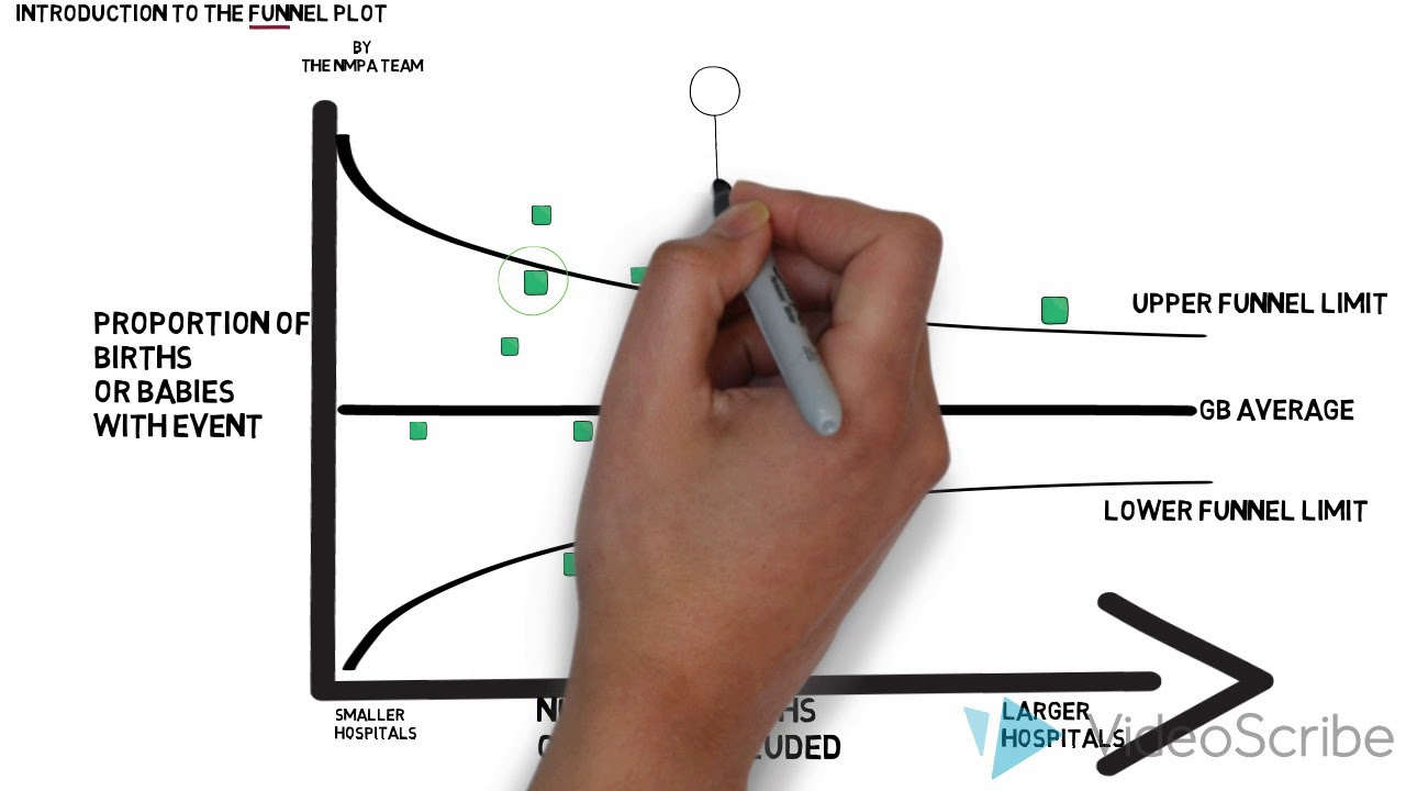
Funnel plot is a specially designed data visualisation for conducting unbiased comparison between outlets, stores or business entities. By the end of this hands-on exercise, you will gain hands-on experience on:
plotting funnel plots by using funnelPlotR package,
plotting static funnel plot by using ggplot2 package, and
plotting interactive funnel plot by using both plotly R and ggplot2 packages.
According to How to read a funnel plot,
The plot should ideally look like a pyramid or a symmetrical inverted funnel, as seen in Image A.
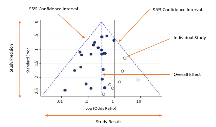
Each included study is represented as a dot.
The y-axis represents a measure of study precision, with standard error being commonly used. Larger studies with greater precision are displayed at the top and studies with lower precision at the bottom. Other measures such as the reciprocal of the standard error, the reciprocal of the sample size, or variance of the estimated effect can also be used as the y-axis.
The x-axis displays the study estimated effect size for an outcome. The scale for the x-axis can include risk ratios or odds ratios (which should be plotted on a logarithmic scale), or continuous measures such as mean difference or standardised mean difference.
In the absence of both bias and heterogeneity, 95% of studies would be expected to lie within the diagonal dotted ‘95% Confidence Interval’ lines, as shown in Figure A.
As a rule of thumb, tests for funnel plot asymmetry should only be used when at least 10 studies are included in the meta-analysis, because the power of the tests is low when there are fewer studies.
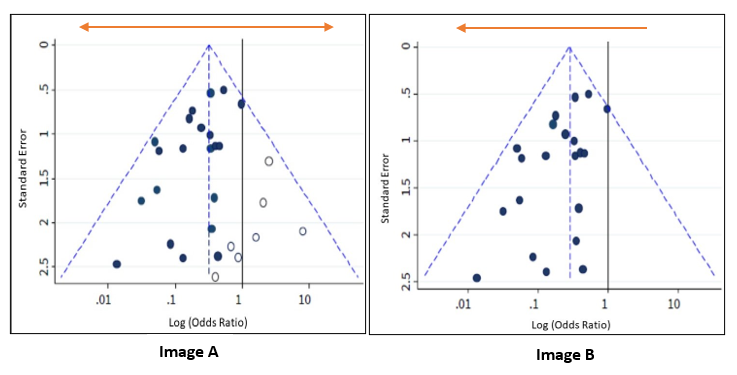
Image A is shown again below alongside Image B, which depicts an asymmetrical funnel due to presence of bias (the points are now predominantly towards the left). In this case, the meta-analysis summary estimate will tend to overestimate the intervention effect. The greater the asymmetry, the greater the likelihood that the amount of bias in the meta-analysis will be significant.
Possible reasons for asymmetry in a funnel plot are:
Non-reporting bias: Some studies, or specific results, are less likely to be published if they are not statistically significant, or if the effect size is very small or non-existent.
Poor methodological quality leading to exaggerated effects: Studies with inferior methods may show larger effect estimates of an intervention than would have been observed in a well-designed study.
True heterogeneity: Sometimes a significant benefit of an intervention can only be observed in patients who are at high risk for the outcome targeted by the intervention. These high-risk patients are more likely to be included in small, early trials, leading to asymmetry in the funnel plot.
Artefactual: Certain effect estimates, such as odds ratios or standardised mean differences, are inherently correlated with their standard errors. This correlation can create a false asymmetry in a funnel plot even when there is no bias.
Chance: With a small number of studies and their heterogeneity (variation), the analysis of the relationships between studies in a meta-analysis is more prone to false positives. This can affect the symmetry of the funnel plot.
The code chunk below uses p_load() of pacman package to check if the following R packages are installed in the computer. If they are, then they will be launched into R.
readr for importing csv into R.
FunnelPlotR for creating funnel plot.
ggplot2 for creating funnel plot manually.
knitr for building static html table.
plotly for creating interactive funnel plot.
pacman::p_load(tidyverse, FunnelPlotR, plotly, knitr)In this section, COVID-19_DKI_Jakarta will be used. The data was downloaded from Open Data Covid-19 Provinsi DKI Jakarta portal. For this hands-on exercise, we are going to compare the cumulative COVID-19 cases and death by sub-district (i.e. kelurahan) as at 31st July 2021, DKI Jakarta.
The code chunk below imports the data into R and save it into a tibble data frame object called covid19.
covid19 <- read_csv("data/COVID-19_DKI_Jakarta.csv") %>%
  mutate_if(is.character, as.factor)
Rows: 267 Columns: 7
── Column specification ────────────────────────────────────────────────────────
Delimiter: ","
chr (3): City, District, Sub-district
dbl (4): Sub-district ID, Positive, Recovered, Death
ℹ Use `spec()` to retrieve the full column specification for this data.
ℹ Specify the column types or set `show_col_types = FALSE` to quiet this message.covid19# A tibble: 267 × 7
`Sub-district ID` City District `Sub-district` Positive Recovered Death
<dbl> <fct> <fct> <fct> <dbl> <dbl> <dbl>
1 3172051003 JAKARTA U… PADEMAN… ANCOL 1776 1691 26
2 3173041007 JAKARTA B… TAMBORA ANGKE 1783 1720 29
3 3175041005 JAKARTA T… KRAMAT … BALE KAMBANG 2049 1964 31
4 3175031003 JAKARTA T… JATINEG… BALI MESTER 827 797 13
5 3175101006 JAKARTA T… CIPAYUNG BAMBU APUS 2866 2792 27
6 3174031002 JAKARTA S… MAMPANG… BANGKA 1828 1757 26
7 3175051002 JAKARTA T… PASAR R… BARU 2541 2433 37
8 3175041004 JAKARTA T… KRAMAT … BATU AMPAR 3608 3445 68
9 3171071002 JAKARTA P… TANAH A… BENDUNGAN HIL… 2012 1937 38
10 3175031002 JAKARTA T… JATINEG… BIDARA CINA 2900 2773 52
# ℹ 257 more rowsFunnelPlotR package uses ggplot to generate funnel plots. It requires a numerator (events of interest), denominator (population to be considered) and group. The key arguments selected for customisation are:
limit: plot limits (95 or 99).
label_outliers: to label outliers (true or false).
Poisson_limits: to add Poisson limits to the plot.
OD_adjust: to add overdispersed limits to the plot.
xrange and yrange: to specify the range to display for axes, acts like a zoom function.
Other aesthetic components such as graph title, axis labels etc.
The code chunk below plots a funnel plot.
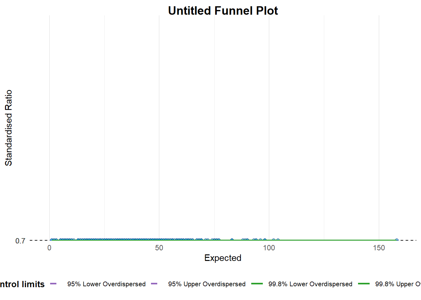
A funnel plot object with 267 points of which 0 are outliers.
Plot is adjusted for overdispersion. funnel_plot(
numerator = covid19$Positive,
denominator = covid19$Death,
group = covid19$`Sub-district`
) Things to learn from the code chunk above:
group in this function is different from the scatterplot. Here, it defines the level of the points to be plotted i.e. Sub-district, District or City. If Cityc is chosen, there are only six data points.
By default, data_typeargument is “SR”.
limit: Plot limits, accepted values are: 95 or 99, corresponding to 95% or 99.8% quantiles of the distribution.
The code chunk below plots a funnel plot.
A funnel plot object with 267 points of which 7 are outliers.
Plot is adjusted for overdispersion. funnel_plot(
numerator = covid19$Death,
denominator = covid19$Positive,
group = covid19$`Sub-district`,
data_type = "PR", #<<
xrange = c(0, 6500), #<<
yrange = c(0, 0.05) #<<
) Things to learn from the code chunk above:
+ data_type argument is used to change from default “SR” to “PR” (i.e. proportions).
+ xrange and yrange are used to set the range of x-axis and y-axis.
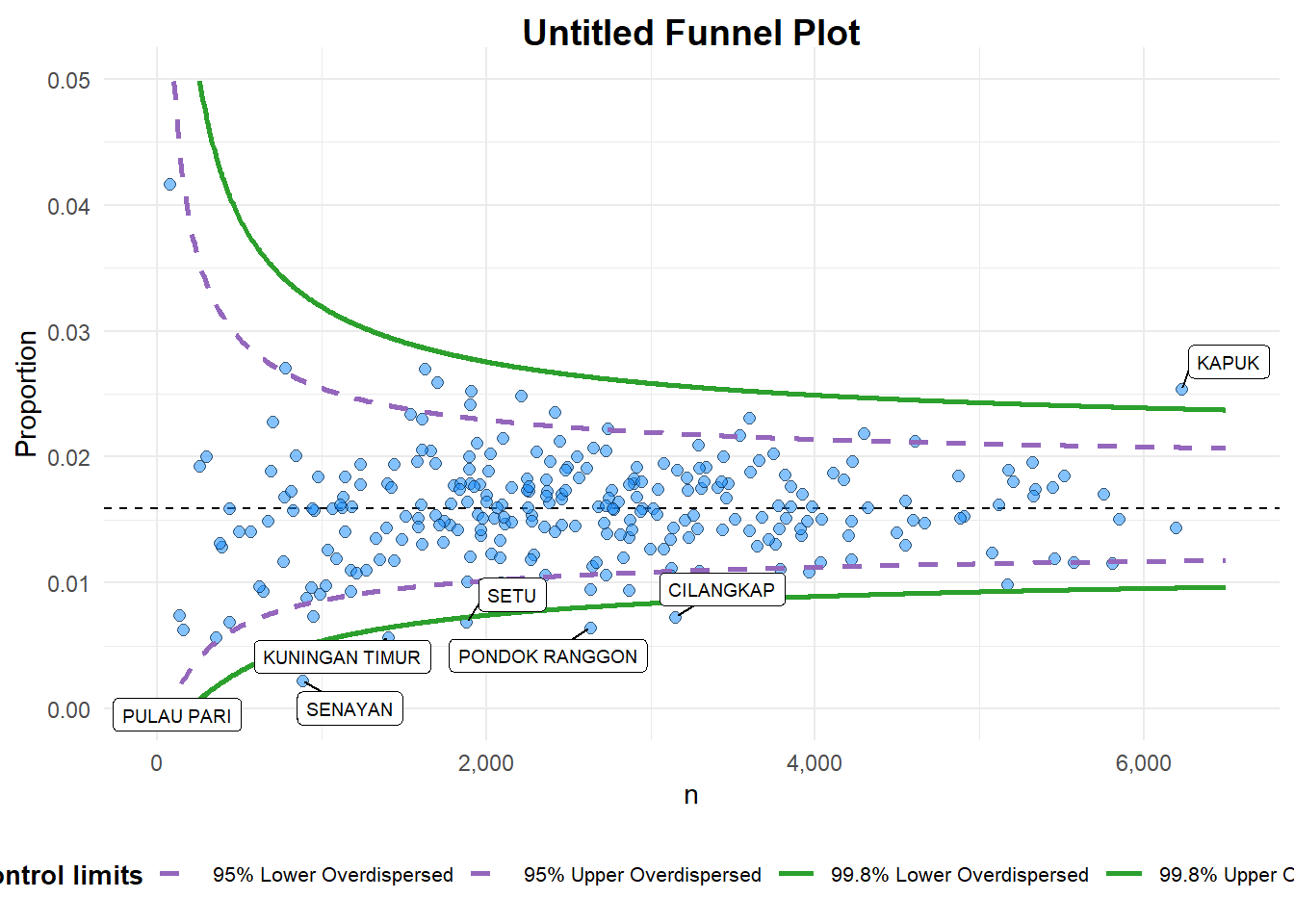
The code chunk below plots a funnel plot.
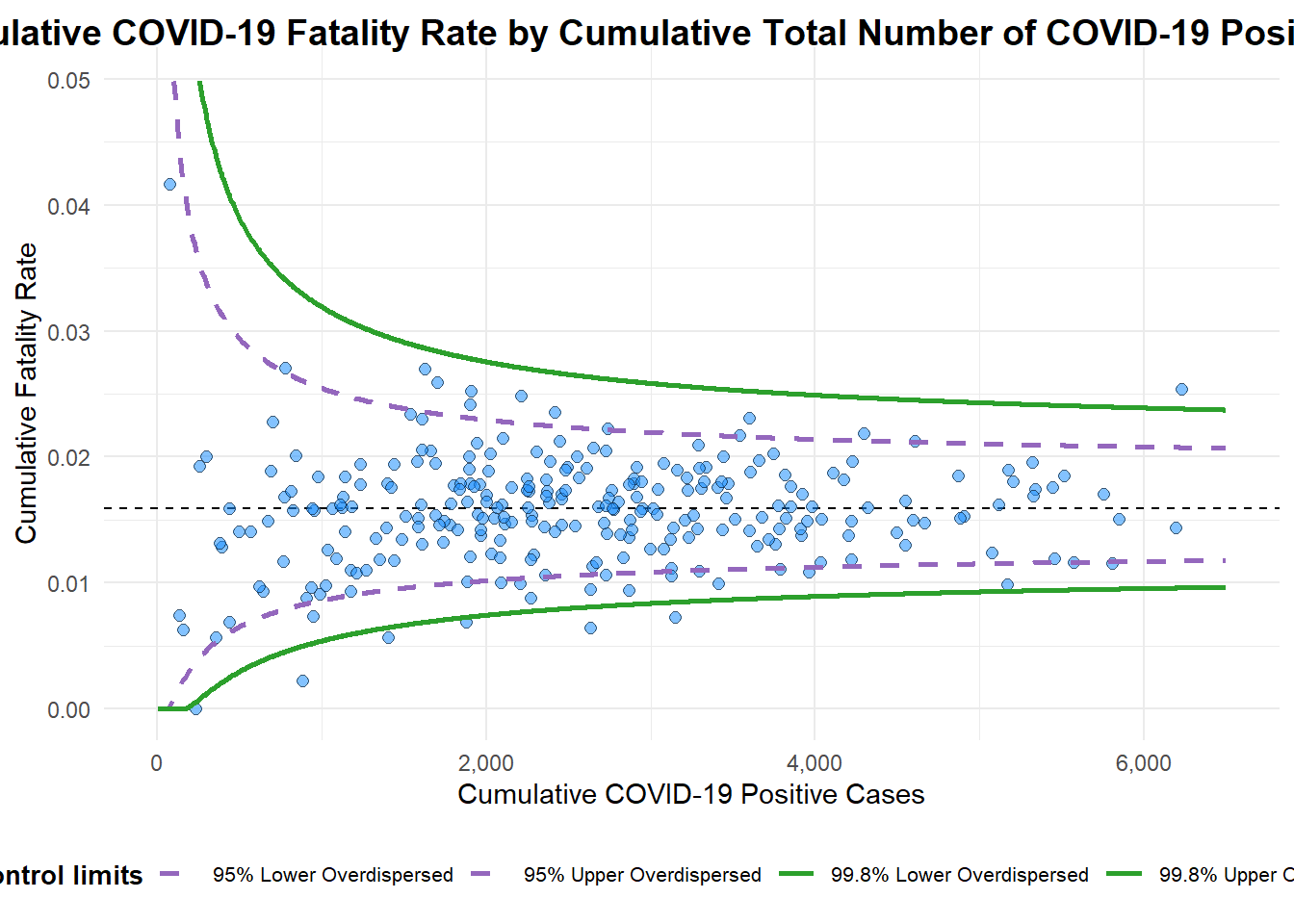
A funnel plot object with 267 points of which 7 are outliers.
Plot is adjusted for overdispersion. funnel_plot(
numerator = covid19$Death,
denominator = covid19$Positive,
group = covid19$`Sub-district`,
data_type = "PR",
xrange = c(0, 6500),
yrange = c(0, 0.05),
label = NA,
title = "Cumulative COVID-19 Fatality Rate by Cumulative Total Number of COVID-19 Positive Cases", #<<
x_label = "Cumulative COVID-19 Positive Cases", #<<
y_label = "Cumulative Fatality Rate" #<<
)Things to learn from the code chunk above:
label = NA argument is to removed the default label outliers feature.
title argument is used to add plot title.
x_label and y_label arguments are used to add/edit x-axis and y-axis titles.
In this section, you will gain hands-on experience on building funnel plots step-by-step by using ggplot2. It aims to enhance you working experience of ggplot2 to customise speciallised data visualisation like funnel plot.
To plot the funnel plot from scratch, we need to derive cumulative death rate and standard error of cumulative death rate.
df <- covid19 %>%
  mutate(rate = Death / Positive) %>%
  mutate(rate.se = sqrt((rate*(1-rate)) / (Positive))) %>%
  filter(rate > 0)
Next, the fit.mean is computed by using the code chunk below.
fit.mean <- weighted.mean(df$rate, 1/df$rate.se^2)The code chunk below is used to compute the lower and upper limits for 95% confidence interval.
number.seq <- seq(1, max(df$Positive), 1)
number.ll95 <- fit.mean - 1.96 * sqrt((fit.mean*(1-fit.mean)) / (number.seq))
number.ul95 <- fit.mean + 1.96 * sqrt((fit.mean*(1-fit.mean)) / (number.seq))
number.ll999 <- fit.mean - 3.29 * sqrt((fit.mean*(1-fit.mean)) / (number.seq))
number.ul999 <- fit.mean + 3.29 * sqrt((fit.mean*(1-fit.mean)) / (number.seq))
dfCI <- data.frame(number.ll95, number.ul95, number.ll999,
number.ul999, number.seq, fit.mean)In the code chunk below, ggplot2 functions are used to plot a static funnel plot.
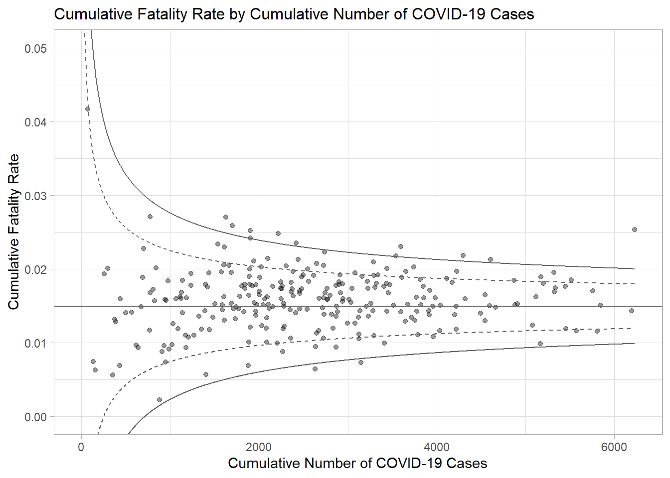
p <- ggplot(df, aes(x = Positive, y = rate)) +
  geom_point(aes(label=`Sub-district`),
             alpha=0.4) +
  geom_line(data = dfCI,
            aes(x = number.seq,
                y = number.ll95),
            size = 0.4,
            colour = "grey40",
            linetype = "dashed") +
  geom_line(data = dfCI,
            aes(x = number.seq,
                y = number.ul95),
            size = 0.4,
            colour = "grey40",
            linetype = "dashed") +
  geom_line(data = dfCI,
            aes(x = number.seq,
                y = number.ll999),
            size = 0.4,
            colour = "grey40") +
  geom_line(data = dfCI,
            aes(x = number.seq,
                y = number.ul999),
            size = 0.4,
            colour = "grey40") +
  geom_hline(data = dfCI,
             aes(yintercept = fit.mean),
             size = 0.4,
             colour = "grey40") +
  coord_cartesian(ylim=c(0,0.05)) +
  annotate("text", x = 1, y = -0.13, label = "95%", size = 3, colour = "grey40") +
  annotate("text", x = 4.5, y = -0.18, label = "99%", size = 3, colour = "grey40") +
  ggtitle("Cumulative Fatality Rate by Cumulative Number of COVID-19 Cases") +
  xlab("Cumulative Number of COVID-19 Cases") +
  ylab("Cumulative Fatality Rate") +
  theme_light() +
  theme(plot.title = element_text(size=12),
        legend.position = c(0.91,0.85),
        legend.title = element_text(size=7),
        legend.text = element_text(size=7),
        legend.background = element_rect(colour = "grey60", linetype = "dotted"),
        legend.key.height = unit(0.3, "cm"))
pThe funnel plot created using ggplot2 functions can be made interactive with ggplotly() of plotly r package.
fp_ggplotly <- ggplotly(p,
  tooltip = c("label",
              "x",
              "y"))
fp_ggplotly