The Big Mac Index (BMI) was invented by The Economist in 1986 as a light-hearted guide to whether currencies are at their “correct” level. It is based on the theory of purchasing-power parity (PPP), with the notion that in the long run, exchange rates should move towards the rate that would equalise the prices of an identical basket of goods and services (in this case, a burger) in any two countries. The BMI has become a global standard, included in several economic textbooks and the subject of dozens of academic studies. Thus, we would like to visually examine the phenomenon of inflation co-movement by looking at the similarities in BMI prices between countries through time, isolate groups with similar characteristics, and determine if the BMI is a suitable proxy to inflation prices.
There is a significant gap in making complex economic data accessible to the general public and providing advanced analysis tools for professionals. Existing visualization tools, including government dashboards, often fail to cater effectively to both audiences. To address this, we propose an R Shiny-based interactive tool that leverages publicly available data, the Big Mac Index to simplify the understanding of global financial trends for laypersons while offering in-depth data exploration and modelling capabilities for analysts.
2 Getting Started
2.1 Installing and loading the required libraries
AER: for functions used in Applied Econometrics with R
CGPfunctions: for using newggslopegraph() for creating slopegraphs
corrplot: provides a visual exploratory tool on correlation matrix that supports automatic variable reordering to help detect hidden patterns among variables.
tidyverse, a family of modern R packages specially designed to support data science, analysis and communication task including creating static statistical graphs
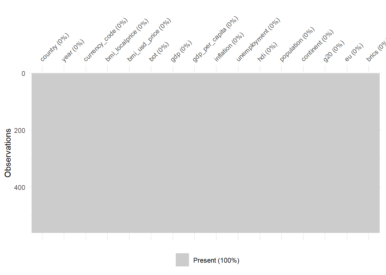
We load the dataset for Big Mac Index that has been combined with other data (e.g. GDP, Employment rates etc.) and the country dataset as seen here in our data preparation. We left join the country dataset to the Big Mac Index dataset.
fun_cat <-function(x) {# Count the number of missing values nmiss <-sum(is.na(x))# Frequency n <-table(x)# Proportion p <-prop.table(n)# Putting it together OUT <-cbind(n, p)# Add nmiss, but first pad to have the right number of rows nmiss <-c(nmiss, rep(NA, nrow(OUT)-1)) OUT <-cbind(OUT, nmiss)return(OUT)}
code block
fun_cat(bmi_data$country)
                n          p nmiss
Argentina      20 0.03571429     0
Australia      20 0.03571429    NA
Brazil         20 0.03571429    NA
Canada         20 0.03571429    NA
Chile          20 0.03571429    NA
China          20 0.03571429    NA
Czech Rep.     20 0.03571429    NA
Denmark        20 0.03571429    NA
Hong Kong      20 0.03571429    NA
Hungary        20 0.03571429    NA
Indonesia      20 0.03571429    NA
Japan          20 0.03571429    NA
Korea          20 0.03571429    NA
Malaysia       20 0.03571429    NA
Mexico         20 0.03571429    NA
New Zealand    20 0.03571429    NA
Peru           20 0.03571429    NA
Philippines    20 0.03571429    NA
Poland         20 0.03571429    NA
Russia         20 0.03571429    NA
Singapore      20 0.03571429    NA
South Africa   20 0.03571429    NA
Sweden         20 0.03571429    NA
Switzerland    20 0.03571429    NA
Thailand       20 0.03571429    NA
Turkey         20 0.03571429    NA
United Kingdom 20 0.03571429    NA
United States  20 0.03571429    NA
code block
fun_cat(bmi_data$currency_code)
     n          p nmiss
ARS 20 0.03571429     0
AUD 20 0.03571429    NA
BRL 20 0.03571429    NA
CAD 20 0.03571429    NA
CHF 20 0.03571429    NA
CLP 20 0.03571429    NA
CNY 20 0.03571429    NA
CZK 20 0.03571429    NA
DKK 20 0.03571429    NA
GBP 20 0.03571429    NA
HKD 20 0.03571429    NA
HUF 20 0.03571429    NA
IDR 20 0.03571429    NA
JPY 20 0.03571429    NA
KRW 20 0.03571429    NA
MXN 20 0.03571429    NA
MYR 20 0.03571429    NA
NZD 20 0.03571429    NA
PEN 20 0.03571429    NA
PHP 20 0.03571429    NA
PLN 20 0.03571429    NA
RUB 20 0.03571429    NA
SEK 20 0.03571429    NA
SGD 20 0.03571429    NA
THB 20 0.03571429    NA
TRY 20 0.03571429    NA
USD 20 0.03571429    NA
ZAR 20 0.03571429    NA
code block
fun_cat(bmi_data$year)
      n    p nmiss
2002 28 0.05     0
2003 28 0.05    NA
2004 28 0.05    NA
2005 28 0.05    NA
2006 28 0.05    NA
2007 28 0.05    NA
2008 28 0.05    NA
2009 28 0.05    NA
2010 28 0.05    NA
2011 28 0.05    NA
2012 28 0.05    NA
2013 28 0.05    NA
2014 28 0.05    NA
2015 28 0.05    NA
2016 28 0.05    NA
2017 28 0.05    NA
2018 28 0.05    NA
2019 28 0.05    NA
2020 28 0.05    NA
2021 28 0.05    NA
code block
fun_cat(bmi_data$continent)
                n          p nmiss
Africa         20 0.03571429     0
Asia          200 0.35714286    NA
Europe        160 0.28571429    NA
North America  60 0.10714286    NA
Oceania        40 0.07142857    NA
South America  80 0.14285714    NA
code block
fun_cat(bmi_data$g20)
          n         p nmiss
g20     260 0.4642857     0
non_g20 300 0.5357143    NA
code block
fun_cat(bmi_data$brics)
            n         p nmiss
brics      80 0.1428571     0
non_brics 480 0.8571429    NA
code block
fun_cat(bmi_data$eu)
         n         p nmiss
eu     100 0.1785714     0
non_eu 460 0.8214286    NA
$bmi_data.bmi_localprice
   Min. 1st Qu.  Median    Mean 3rd Qu.    Max.
      2       6      18   22010      83 4000000

$bmi_data.bmi_usd_price
   Min. 1st Qu.  Median    Mean 3rd Qu.    Max.
 0.7987  2.2978  2.9915  3.2198  4.0036  8.0630

$bmi_data.bot
      Min.    1st Qu.     Median       Mean    3rd Qu.       Max.
-1.588e+09 -2.980e+07  5.006e+06 -3.000e+07  2.714e+07  9.638e+08

$bmi_data.gdp
     Min.   1st Qu.    Median      Mean   3rd Qu.      Max.
5.478e+10 2.450e+11 4.765e+11 1.664e+12 1.335e+12 2.330e+13

$bmi_data.gdp_per_capita
   Min. 1st Qu.  Median    Mean 3rd Qu.    Max.
  888.9  7199.9 14138.8 24770.2 42106.0 93446.4

$bmi_data.inflation
   Min. 1st Qu.  Median    Mean 3rd Qu.    Max.
 -2.983   1.388   2.526   3.824   4.392  53.550

$bmi_data.hdi
   Min. 1st Qu.  Median    Mean 3rd Qu.    Max.
 0.6040  0.7540  0.8455  0.8294  0.9113  0.9620

$bmi_data.population
     Min.   1st Qu.    Median      Mean   3rd Qu.      Max.
3.949e+06 1.027e+07 3.862e+07 1.139e+08 1.068e+08 1.426e+09
code block
# Assuming 'bmi_data' is your data frameresult_list <-lapply(split(bmi_data, bmi_data$year),function(sub_data) summary(sub_data$bmi_usd_price))result_list
$`2002`
   Min. 1st Qu.  Median    Mean 3rd Qu.    Max.
 0.7987  1.3816  1.6921  1.9122  2.3643  3.7952

$`2003`
   Min. 1st Qu.  Median    Mean 3rd Qu.    Max.
  1.196   1.480   1.956   2.142   2.298   4.599

$`2004`
   Min. 1st Qu.  Median    Mean 3rd Qu.    Max.
  1.234   1.606   2.157   2.288   2.577   4.884

$`2005`
   Min. 1st Qu.  Median    Mean 3rd Qu.    Max.
  1.269   1.615   2.440   2.466   2.660   5.050

$`2006`
   Min. 1st Qu.  Median    Mean 3rd Qu.    Max.
  1.302   1.593   2.579   2.541   2.990   4.931

$`2007`
   Min. 1st Qu.  Median    Mean 3rd Qu.    Max.
  1.415   2.097   2.697   2.754   3.090   5.046

$`2008`
   Min. 1st Qu.  Median    Mean 3rd Qu.    Max.
  1.699   2.465   3.278   3.469   4.378   6.375

$`2009`
   Min. 1st Qu.  Median    Mean 3rd Qu.    Max.
  1.716   2.139   3.047   3.089   3.621   5.985

$`2010`
   Min. 1st Qu.  Median    Mean 3rd Qu.    Max.
  1.831   2.315   3.184   3.309   3.838   6.304

$`2011`
   Min. 1st Qu.  Median    Mean 3rd Qu.    Max.
  1.938   2.772   3.713   3.952   4.519   8.063

$`2012`
   Min. 1st Qu.  Median    Mean 3rd Qu.    Max.
  2.124   2.576   3.628   3.676   4.278   6.806

$`2013`
   Min. 1st Qu.  Median    Mean 3rd Qu.    Max.
  2.191   2.906   3.769   3.886   4.453   7.125

$`2014`
   Min. 1st Qu.  Median    Mean 3rd Qu.    Max.
  2.160   2.884   3.518   3.723   4.498   7.142

$`2015`
   Min. 1st Qu.  Median    Mean 3rd Qu.    Max.
  1.364   2.882   3.348   3.618   4.331   7.544

$`2016`
   Min. 1st Qu.  Median    Mean 3rd Qu.    Max.
  1.527   2.632   3.084   3.246   3.786   6.443

$`2017`
   Min. 1st Qu.  Median    Mean 3rd Qu.    Max.
  1.789   2.629   3.301   3.431   4.195   6.350

$`2018`
   Min. 1st Qu.  Median    Mean 3rd Qu.    Max.
  2.276   2.789   3.766   3.833   4.535   6.765

$`2019`
   Min. 1st Qu.  Median    Mean 3rd Qu.    Max.
  1.652   2.549   3.657   3.555   4.296   6.622

$`2020`
   Min. 1st Qu.  Median    Mean 3rd Qu.    Max.
  2.154   2.770   3.560   3.651   4.420   6.713

$`2021`
   Min. 1st Qu.  Median    Mean 3rd Qu.    Max.
  1.809   2.886   3.863   3.854   4.547   7.291
code block
# Assuming 'bmi_data' is your data frameresult_list <-lapply(split(bmi_data, bmi_data$country),function(sub_data) summary(sub_data$bmi_usd_price))result_list
$Argentina
   Min. 1st Qu.  Median    Mean 3rd Qu.    Max.
 0.7987  1.7920  2.9321  2.8030  3.6693  4.8397

$Australia
   Min. 1st Qu.  Median    Mean 3rd Qu.    Max.
  1.613   2.667   4.127   3.711   4.532   4.985

$Brazil
   Min. 1st Qu.  Median    Mean 3rd Qu.    Max.
  1.482   2.935   4.639   4.061   5.140   6.162

$Canada
   Min. 1st Qu.  Median    Mean 3rd Qu.    Max.
  2.121   3.069   4.327   4.046   5.031   5.394

$Chile
   Min. 1st Qu.  Median    Mean 3rd Qu.    Max.
  1.955   2.972   3.268   3.304   3.916   4.346

$China
   Min. 1st Qu.  Median    Mean 3rd Qu.    Max.
  1.196   1.387   2.356   2.215   2.784   3.459

$`Czech Rep.`
   Min. 1st Qu.  Median    Mean 3rd Qu.    Max.
  1.655   2.556   3.461   3.200   3.769   4.558

$Denmark
   Min. 1st Qu.  Median    Mean 3rd Qu.    Max.
  2.953   4.464   4.862   4.846   5.375   5.994

$`Hong Kong`
   Min. 1st Qu.  Median    Mean 3rd Qu.    Max.
  1.400   1.547   2.031   2.039   2.476   2.643

$Hungary
   Min. 1st Qu.  Median    Mean 3rd Qu.    Max.
  1.688   2.686   3.045   3.149   3.666   4.644

$Indonesia
   Min. 1st Qu.  Median    Mean 3rd Qu.    Max.
  1.530   1.823   2.241   2.166   2.409   2.860

$Japan
   Min. 1st Qu.  Median    Mean 3rd Qu.    Max.
  2.015   2.337   3.200   3.074   3.522   4.160

$Korea
   Min. 1st Qu.  Median    Mean 3rd Qu.    Max.
  2.377   2.715   3.301   3.270   3.704   4.115

$Malaysia
   Min. 1st Qu.  Median    Mean 3rd Qu.    Max.
  1.326   1.545   1.980   1.931   2.290   2.579

$Mexico
   Min. 1st Qu.  Median    Mean 3rd Qu.    Max.
  2.069   2.470   2.656   2.626   2.750   3.350

$`New Zealand`
   Min. 1st Qu.  Median    Mean 3rd Qu.    Max.
  1.607   3.149   3.980   3.709   4.346   4.874

$Peru
   Min. 1st Qu.  Median    Mean 3rd Qu.    Max.
  2.283   2.761   3.189   3.112   3.400   3.907

$Philippines
   Min. 1st Qu.  Median    Mean 3rd Qu.    Max.
  1.234   1.690   2.657   2.315   2.791   3.670

$Poland
   Min. 1st Qu.  Median    Mean 3rd Qu.    Max.
  1.460   2.247   2.533   2.537   2.949   3.514

$Russia
   Min. 1st Qu.  Median    Mean 3rd Qu.    Max.
  1.250   1.515   1.945   1.958   2.361   2.702

$Singapore
   Min. 1st Qu.  Median    Mean 3rd Qu.    Max.
  1.813   2.306   3.398   3.205   3.787   4.433

$`South Africa`
   Min. 1st Qu.  Median    Mean 3rd Qu.    Max.
 0.8899  2.0453  2.1739  2.1354  2.2983  2.8735

$Sweden
   Min. 1st Qu.  Median    Mean 3rd Qu.    Max.
  2.500   4.478   5.353   5.266   6.164   7.640

$Switzerland
   Min. 1st Qu.  Median    Mean 3rd Qu.    Max.
  3.795   5.049   6.401   6.191   6.885   8.063

$Thailand
   Min. 1st Qu.  Median    Mean 3rd Qu.    Max.
  1.270   1.695   2.405   2.516   3.155   4.248

$Turkey
   Min. 1st Qu.  Median    Mean 3rd Qu.    Max.
  1.997   2.706   3.148   3.198   3.762   4.777

$`United Kingdom`
   Min. 1st Qu.  Median    Mean 3rd Qu.    Max.
  2.885   3.614   3.863   3.908   4.379   4.627

$`United States`
   Min. 1st Qu.  Median    Mean 3rd Qu.    Max.
  2.350   2.835   3.725   3.666   4.343   4.890
3 Exploratory Data Analysis
code block
flowchart TB
  A[Year]
  B[Country]
  C[Big Mac Index price]
  D[Inflation rate]
  E[GDP per capita]
  F[Balance of Trade]
  G[Unemployment rate]
  H[Human Development Index]
  I[Population size]

  A --> C
  B --> C
  C --> D
  C --> E
  C --> F
  C --> G
  C --> H
  C --> I
flowchart TB
  A[Year]
  B[Country]
  C[Big Mac Index price]
  D[Inflation rate]
  E[GDP per capita]
  F[Balance of Trade]
  G[Unemployment rate]
  H[Human Development Index]
  I[Population size]

  A --> C
  B --> C
  C --> D
  C --> E
  C --> F
  C --> G
  C --> H
  C --> I
Some questions of interest regarding the problem statement of inflation co-movement by BMI are:
what type of variation occurs within BMI prices,
what type of covariation occurs between BMI prices by dimensions.
To do this, we will look at the following variables:
bmi_usd_price (in order to compare across currencies, we use the BMI prices converted to USD)
by dimensions
country
year
3.1 Univariate Analysis: Looking at BMI
code block
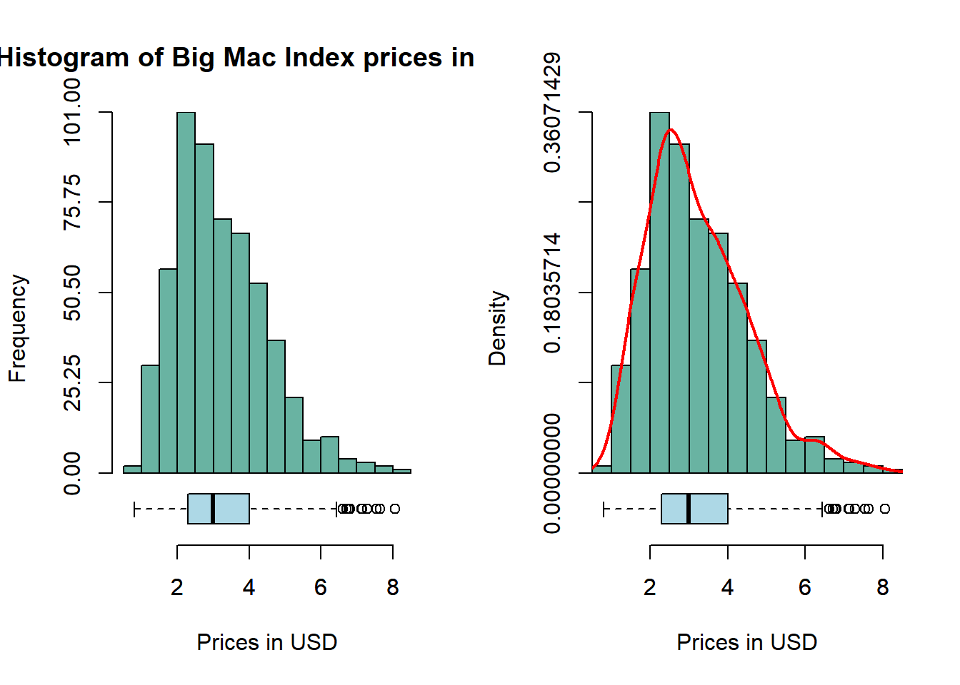
par(mfrow =c(1, 2))hist_boxplot(bmi_data$bmi_usd_price,col="#69b3a2",freq=TRUE, xlab ="Prices in USD", main ="Histogram of Big Mac Index prices in USD")hist_boxplot(bmi_data$bmi_usd_price,col="#69b3a2",freq=FALSE,density=TRUE, xlab ="Prices in USD", main ="")
Insights
BMI is asymmetrically distributed and skewed to the right. Most of the Big Mac prices (adjusted to USD) are close to 3USD - this makes sense as McDonald’s positions itself as an ultra-affordable fast food chain. Its mean (3.2198) is higher than its median (2.9915). But this also means that it has outliers with very expensive Big Mac prices.
Questions:
Why are the Big Mac prices close to 3USD?
Given McDonald’s strategy to be ultra-affordable, why is there a large spread in Big Mac prices and outliers on the right?
3.2 Looking at BMI through individual dimensions
3.2.1 Country dimension with Violin+Boxplot
code block
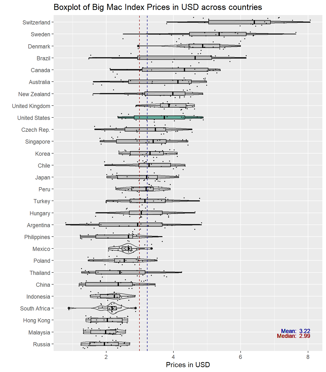
bmi_data %>%# Calculate mean of bmi_usd_price for each countrygroup_by(country) %>%mutate(median_bmi =median(bmi_usd_price)) %>%ungroup() %>%# Reorder the countries based on the mean of bmi_usd_pricemutate(country =reorder(country, median_bmi)) %>%# Add a column called 'type': do we want to highlight the group or not?mutate(type =ifelse(country=="United States", "Highlighted", "Normal")) %>%# Build the boxplot. ggplot(aes(x = country, y = bmi_usd_price, fill = type, alpha = type)) +geom_violin(width=1.0) +geom_boxplot(width=0.3, color="black", alpha=0.8) +geom_jitter(color ="black", size =0.4, alpha =0.9) +scale_fill_manual(values =c("#69b3a2", "grey")) +scale_alpha_manual(values =c(1, 0.1)) +theme(legend.position ="none") +labs(y ="Prices in USD", x ="", title ="Boxplot of Big Mac Index Prices in USD across countries") +coord_flip() +# Add mean and median linesgeom_hline(aes(yintercept =mean(bmi_usd_price), linetype ="Mean"), color ="darkblue", linetype ="dashed", size =0.5) +geom_hline(aes(yintercept =median(bmi_usd_price), linetype ="Median"), color ="darkred", linetype ="dashed", size =0.5) +# Add text labels for mean and mediangeom_text(aes(x =mean(bmi_usd_price), label =paste("Mean: ", round(mean(bmi_usd_price), 2))),y =max(bmi_data$bmi_usd_price, na.rm =TRUE), size =3, vjust =3.5, hjust =1, color ="darkblue") +geom_text(aes(x =median(bmi_usd_price), label =paste("Median: ", round(median(bmi_usd_price), 2))),y =max(bmi_data$bmi_usd_price, na.rm =TRUE), size =3, vjust =4, hjust =1, color ="darkred") +# Customize legendscale_linetype_manual(name ="Lines", values =c("Mean"="dashed", "Median"="dashed"),labels =c("Mean", "Median")) +guides(fill =guide_legend(override.aes =list(alpha =c(1, 0.1))))
Insights
Some of the outliers pointed out in the previous data visualisations can be explained by the country dimension. Highly developed countries such as Switzerland, Sweden and Denmark have the top 3 most expensive Big Mac prices. However, Hong Kong, with also a highly developed economy, has the third lowest Big Mac price. In the boxplot above, there is no clear difference between developed and developing countries (even Philippines is more expensive than Hong Kong).
The above boxplot also shows that there is variation within and between countries - there are some countries with greater variability e.g. Argentina and a number of countries with median BMI prices higher than the overall median BMI price such as Switzerland, Brazil and Canada while countries like Mexico and South Africa (somewhat bimodal) did not see much fluctuations in their BMI prices.
Questions:
Why do some countries have greater variability in their BMI prices?
Why is there a difference in BMI prices between developed and developing countries?
especially for Hong Kong
3.2.2 Year dimension with Violin+Boxplot
code block
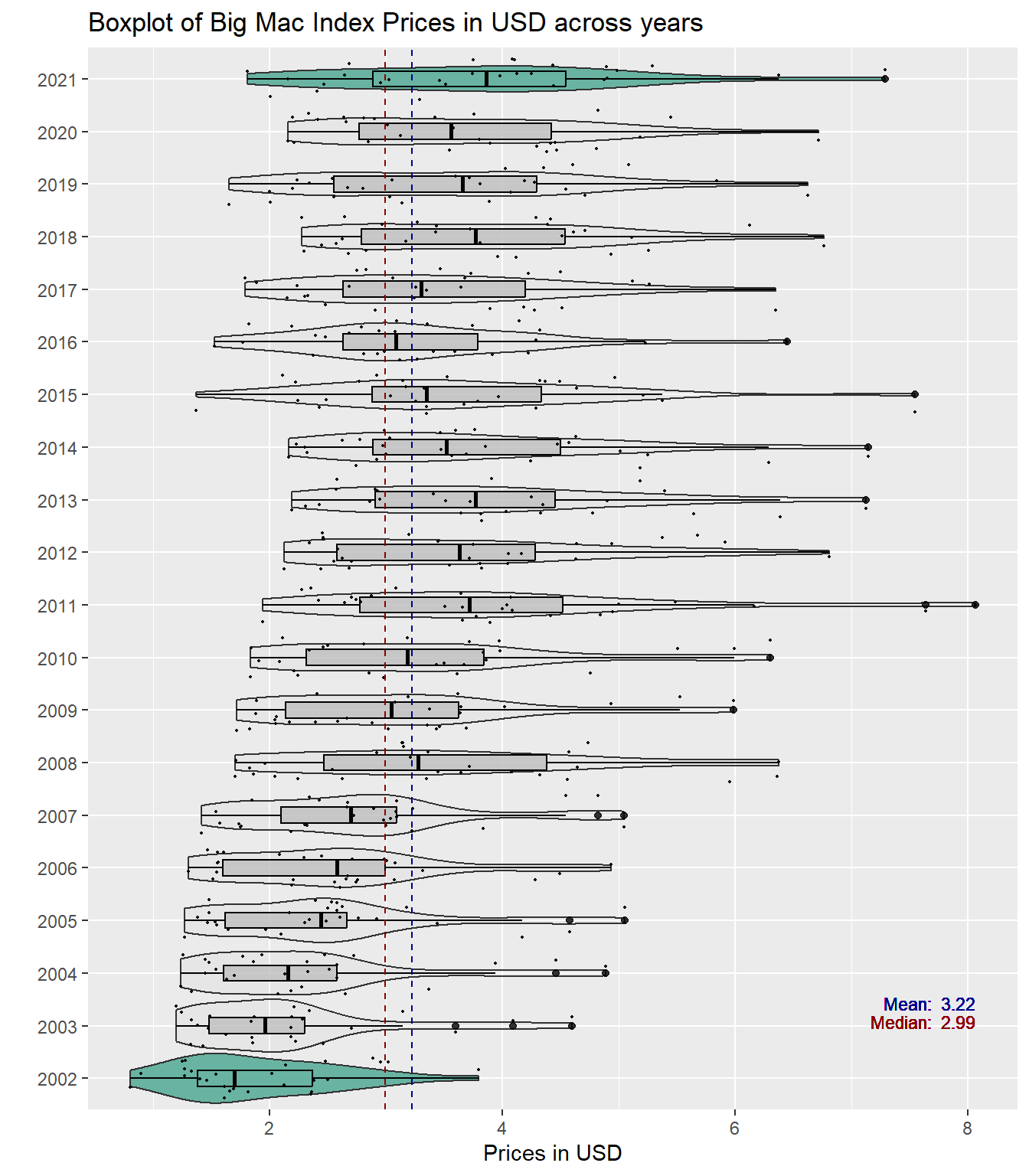
bmi_data %>%mutate(year =factor(year)) %>%# Add a column called 'type': do we want to highlight the group or not?mutate( type=ifelse(year %in%c("2002", "2021"),"Highlighted","Normal")) %>%# Build the boxplot. In the 'fill' argument, give this columnggplot( aes(x=year, y=bmi_usd_price, fill=type, alpha=type)) +geom_violin(width=1.0) +geom_boxplot(width=0.3, color="black", alpha=0.8) +geom_jitter(color ="black", size =0.4, alpha =0.9) +scale_fill_manual(values=c("#69b3a2", "grey")) +scale_alpha_manual(values=c(1,0.1)) +theme(legend.position ="none") +labs(y ="Prices in USD", x ="", title ="Boxplot of Big Mac Index Prices in USD across years") +coord_flip() +# Add mean and median linesgeom_hline(aes(yintercept =mean(bmi_usd_price), linetype ="Mean"), color ="darkblue", linetype ="dashed", size =0.5) +geom_hline(aes(yintercept =median(bmi_usd_price), linetype ="Median"), color ="darkred", linetype ="dashed", size =0.5) +# Add text labels for mean and mediangeom_text(aes(x =mean(bmi_usd_price), label =paste("Mean: ", round(mean(bmi_usd_price), 2))),y =max(bmi_data$bmi_usd_price, na.rm =TRUE), size =3, vjust =3.5, hjust =1, color ="darkblue") +geom_text(aes(x =median(bmi_usd_price), label =paste("Median: ", round(median(bmi_usd_price), 2))),y =max(bmi_data$bmi_usd_price, na.rm =TRUE), size =3, vjust =4, hjust =1, color ="darkred") +# Customize legendscale_linetype_manual(name ="Lines", values =c("Mean"="dashed", "Median"="dashed"),labels =c("Mean", "Median")) +guides(fill =guide_legend(override.aes =list(alpha =c(1, 0.1))))
Insights
From the boxplot above, we can see that Big Mac prices have risen through the years - 2021 is the most expensive year for Big Mac prices. Moreover from 2002 - 2007, according to the violin plot, it seemed that the prices were mostly concentrated but there is more spread since 2008. Despite the blip from 2013 - 2016 and 2018 - 2020, which saw falling Big Mac prices, as a whole, they have increased since 2002 which saw the lowest prices for Big Mac.
Questions:
Why was there a dip in Big Mac prices from 2013 to 2016 and 2018 to 2020?
Why are Big Mac prices rising as a whole?
3.3 Looking at BMI through both dimensions
3.3.1 Plotting a Coplot plot to determine if there is a third variable influence
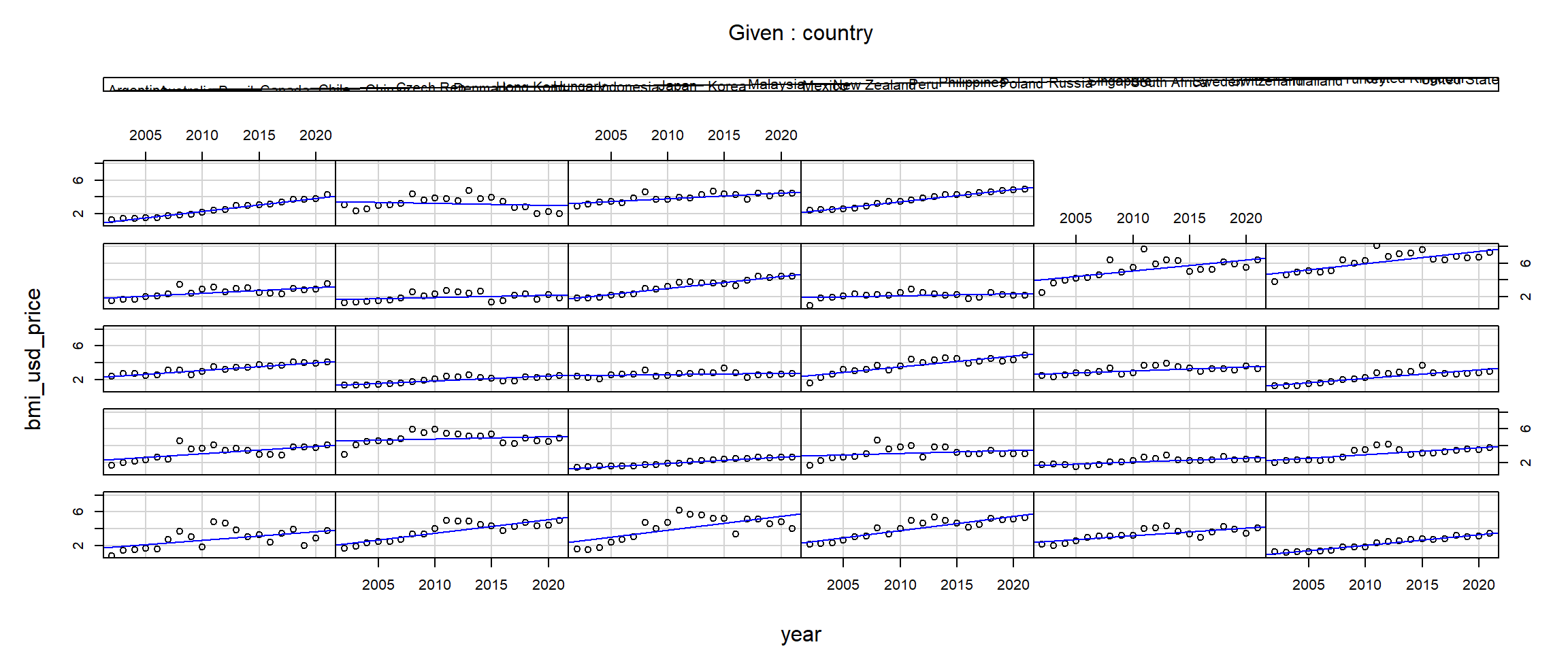
The BMI price in USD is plotted on the y axis and the years are on the x axis. The 28 plots show the relationship between these two variables by each country. The bars at the top indicate the countries position from left to right, starting from the bottom row.
code block
coplot(bmi_usd_price ~ year|country, data = bmi_data, panel =function(x, y, ...) { points(x, y, ...) abline(lm(y ~ x), col ="blue")})
Note
Insights
From the coplots above, there is an interaction between years and countries. Conditionally on country, the relationship between BMI price in USD and year looks roughly linear - the regression results for most countries indicate a positive relationship throughout the years. However, countries like Hong Kong(11), Mexico(15), Russia(20) and South Africa(22) have almost flat regression lines that suggest a weak or almost no relationship between the variables. Moreover, Turkey(26) is the only country with a negative relationship.
4 Time-series Analysis of Big Mac Index through time and countries
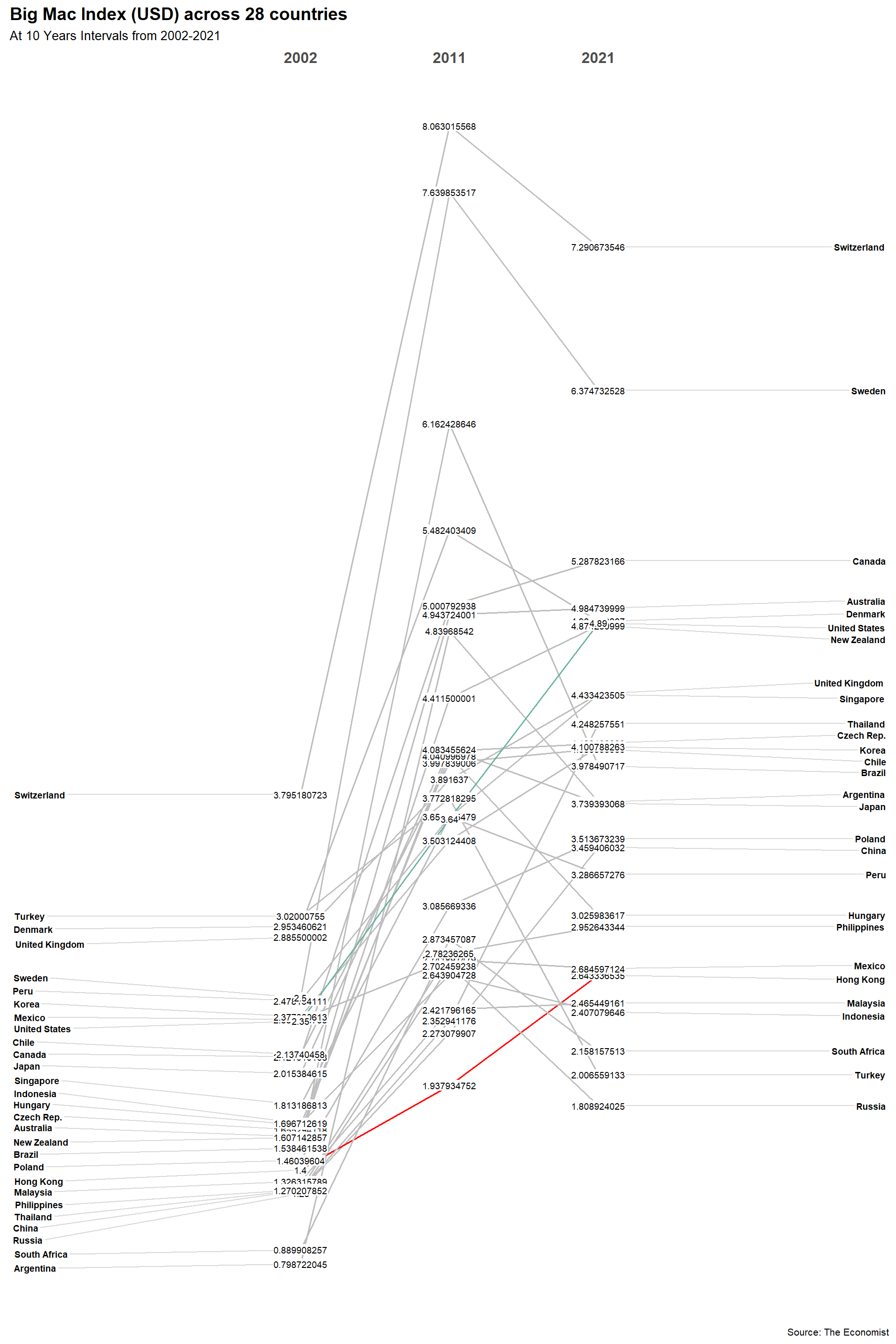
4.1 Looking at overall trends with newsslopegraph()
code block
bmi_data %>%mutate(year =factor(year)) %>%filter(year %in%c(2002, 2011, 2021 )) %>%newggslopegraph(year, bmi_usd_price, country,Title ="Big Mac Index (USD) across 28 countries",SubTitle ="At 10 Years Intervals from 2002-2021",Caption ="Source: The Economist",YTextSize =2.5,LineThickness = .6,LineColor =c(rep("gray",8), "red", rep("gray",18), "#69b3a2"),WiderLabels =TRUE)
Insights
From the slopegraph above, we can see that Big Mac prices increased for all countries in 2011 but later increased for some and decreased for others. Switzerland consistently had the most expensive Big Mac prices through the years while Argentina had the cheapest Big Mac in 2002 but is in 15th position (out of 28) in 2021. Most interesting is Hong Kong, that saw a consistent rise in Big Mac process, did not experience sharp changes, and had actually the cheapest Big Mac in 2011.
Moreover, in 2002, the prices between countries were much closer in spread but this spread increased through the years.
Questions:
Why did the spread in Big Mac prices between countries increase through the years?
Why did Big Mac prices increase in 2011 for all countries?
Why did some countries experience a consistent increase in Big Mac prices while others experienced fluctuations?
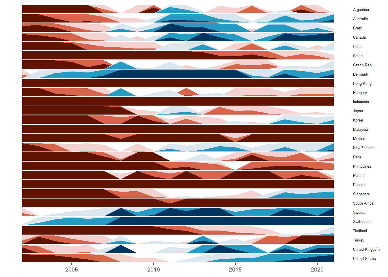
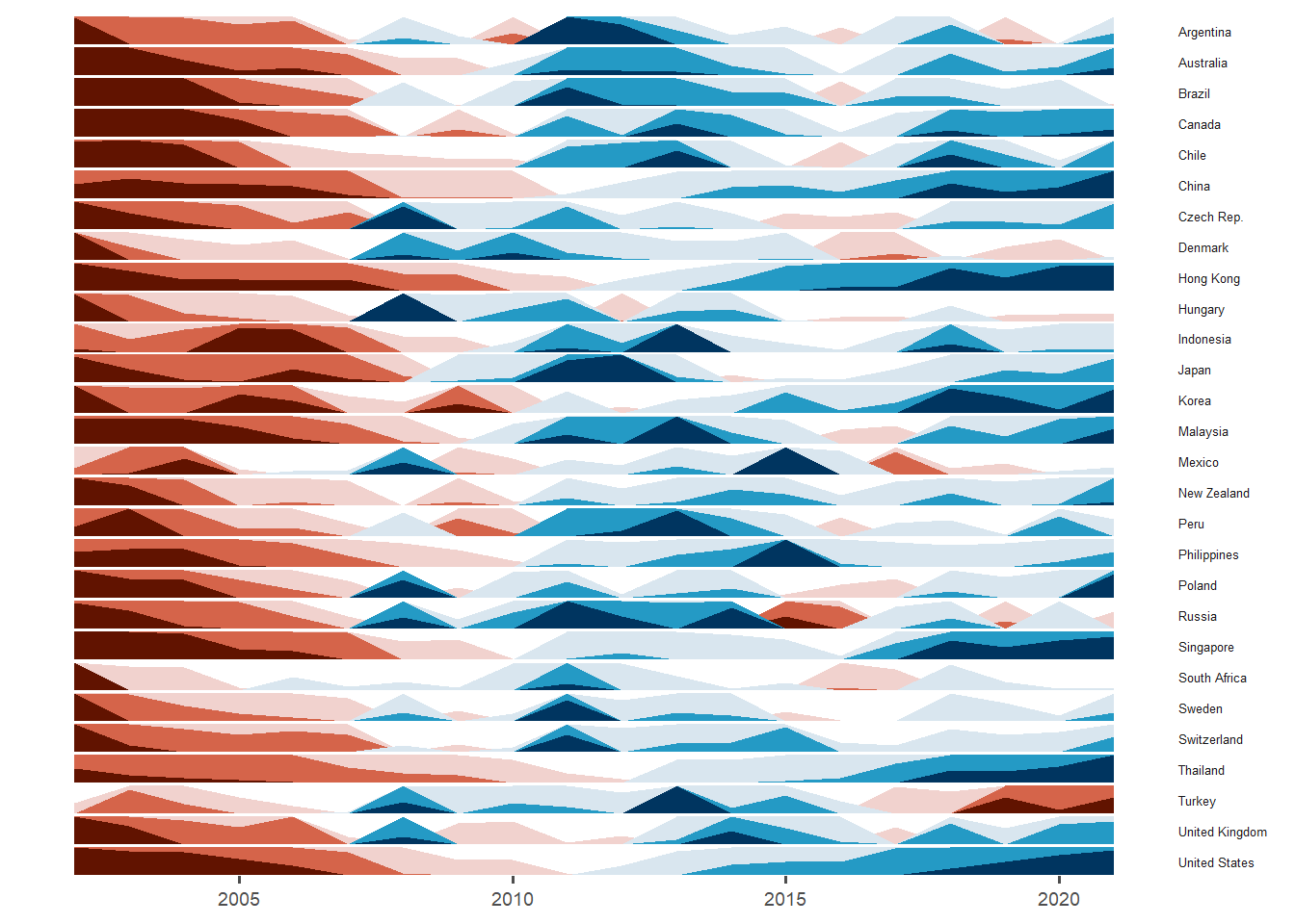
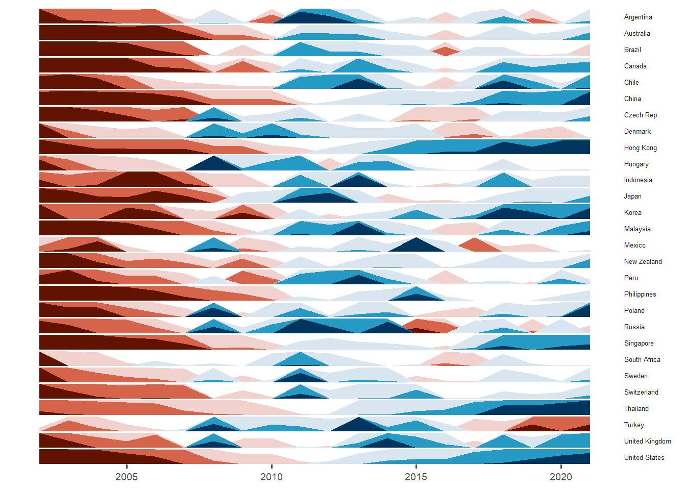
4.2 Looking at variations in patterns with ggHoriPlot()
Toggle the different tabsets to see the different horizon plots.
If US mean bmi_usd_price is used as the origin, Switzerland (and shortly after) Denmark have always had stronger prices than the overall mean Big Mac Index price for USA. China, Hong Kong, Indonesian, Malaysia, Mexico, Philippines, Poland, Russia, South Africa and Turkey have always been weaker in Big Mac prices than the USA.
The horizon plot (using median bmi_usd_price as the baseline) showed that all countries were initially below the median Big Mac price and all experienced some increase in price. China, Hong Kong, Korea, Singapore, Thailand and United States had a huge increase in Big Mac prices around 2018 to 2022. However, Turkey experienced a large drop in recent years while Russia experienced huge increase and than a large drop around 2015 and only had a smaller increase later on.
Questions:
Why do some countries experience a significant increase in Big Mac prices together over the same period?
Why are there small sharp peaks for some years and long peaks for others?
What other factors account for this co-movement in Big Mac prices? GDP per capita?
4.3 Adding GDP per capita to track the movement of BMI through the years, countries (colour) and population (size) with a Bubble Plot
code block
bmi_data %>%plot_ly(x =~gdp_per_capita, y =~bmi_usd_price, size =~population, color =~country,sizes =c(20, 150),frame =~year, text =~paste(country, "<br>Population: ", gdp_per_capita, "<br>Big Mac Price: USD$", bmi_usd_price,"<br>GDP per Capita: $", gdp_per_capita, "<br>Inflation: ", inflation, "%"), hoverinfo ="text",type ='scatter',mode ='markers' ) %>%layout(showlegend =FALSE,xaxis =list(title ="GDP per Capita"),yaxis =list(title ="Price in USD"),title ="A Bubbleplot of Big Mac Index (USD) across 28 countries (colour) with population (size) through the years")
Insights
At the start, it seemed like there was a relationship between GDP per capita and BMI prices - the higher one’s GDP per capita was, the higher the Big Mac price in USD. Switzerland with the highest GDP per capita also saw the most expensive Big Mac prices. The only exception is Hong Kong that had a small inflation rate throughout. For those with higher GDP per capita, their inflation rates were almost the same. While countries with higher GDP per capita above 40k saw their GDP per capita increasing with Big Mac prices consistently above USD$3 since 2010, countries with GDP per capita below 20k saw small increases in their GDP per capita, still remained below 20k while Big Mac prices had a wider variability. Also, most of the countries in our study are of the similar population size.
Questions:
There seems to be two different trajectory of BMI prices for countries with different GDP per capita. Are there other factors influencing this? Are there other trajectories that can be seen?
We have been mostly looking at country and year effects. Are there other variables that affect BMI as a whole?
5 Multivariate Analysis of Big Mac Index through time and countries
5.1 Plotting a Parallel Coordinates plot to see relationships between variables
Based on the parallel coordinates plot, there appears to be interesting patterns. For example, countries lower gdp_per-capita, higher balance of trade (net export - net import) with low inflation and unemployment, and big population sizes had low Big Mac Index prices. Countries with high gdp_per_capita with high human development index (HDI) and small population sizes had very high Big Mac Index prices.
Questions:
What are the correlations between variables with BMI in USD prices?
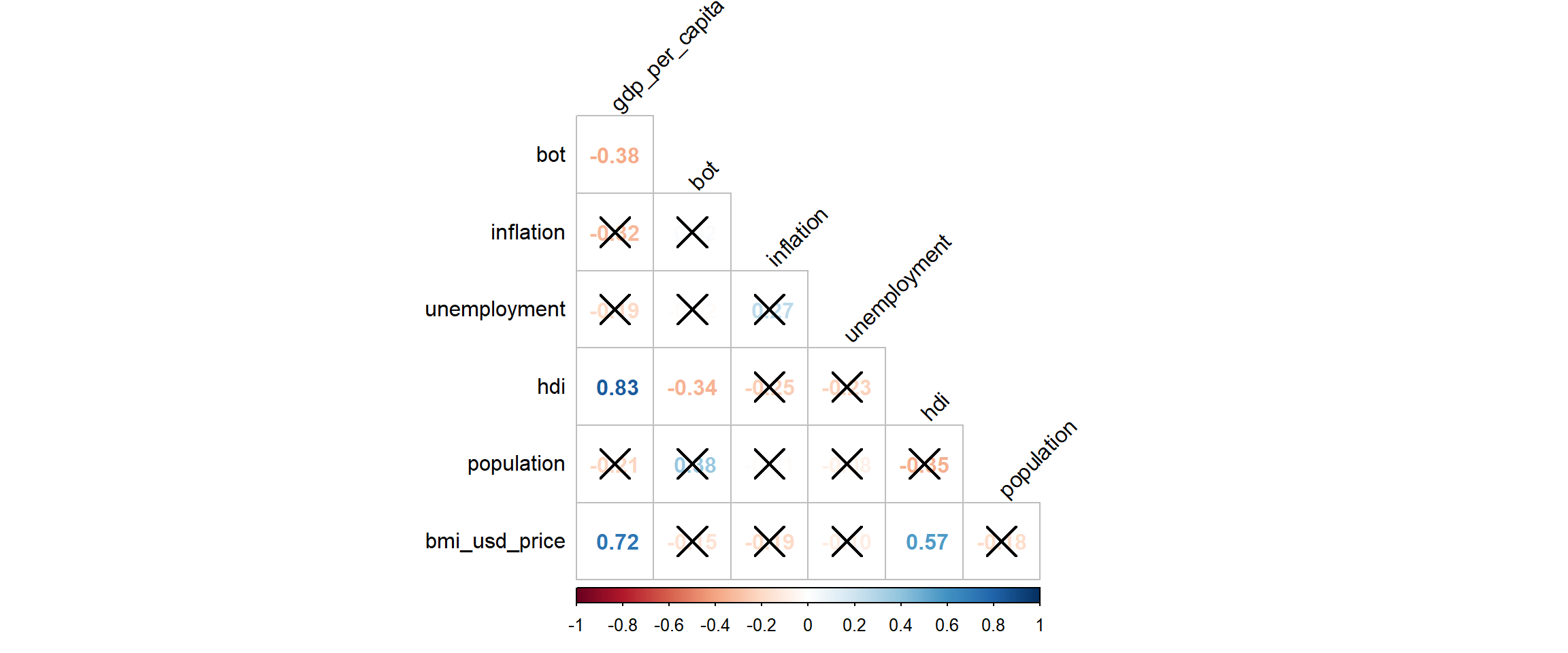
5.2 Plotting a Correlation plot to see correlations between variables
GDP per capita, inflation and Human Development Index are significantly correlated to Big Mac Index prices. Interestingly, even though we had initially posited that inflation and Big Mac prices are correlated, it appears that they are not - inflation is not correlated to Big Mac Index prices. However, we cannot tell if there is a year/country effect - there is no information on the correlation even though though these variables are constant in the time dimension and across countries.
6 Panel Data Regression
Given the time-series (by 20 years) and cross sectionality (by 28 countries) of our data, panel data regression is a good technique to analyze the relationship between our independent variables and Big Mac Index price.
Homogeneous (or pooled) panel data models assume that the model parameters are common across individuals.
Thus, the basic OLS regression model does not consider heterogeneity across countries or years.
code block
ols <-lm(bmi_usd_price ~ gdp_per_capita + hdi, data = bmi_data)summary(ols)
Call:
lm(formula = bmi_usd_price ~ gdp_per_capita + hdi, data = bmi_data)

Residuals:
    Min      1Q  Median      3Q     Max
-1.8586 -0.5952 -0.0552  0.5463  3.3407

Coefficients:
                 Estimate Std. Error t value Pr(>|t|)
(Intercept)     3.401e+00  5.434e-01   6.259 7.74e-10 ***
gdp_per_capita  4.921e-05  3.152e-06  15.608  < 2e-16 ***
hdi            -1.688e+00  7.302e-01  -2.312   0.0211 *
---
Signif. codes:  0 '***' 0.001 '**' 0.01 '*' 0.05 '.' 0.1 ' ' 1

Residual standard error: 0.8813 on 557 degrees of freedom
Multiple R-squared:  0.528, Adjusted R-squared:  0.5263
F-statistic: 311.6 on 2 and 557 DF,  p-value: < 2.2e-16
code block
ggPredict(ols,interactive=TRUE)
Note
Insights
Each point represents observations of GDP per capita, HDI and BMI price in USD - the multiple regression results indicate a positive relationship throughout the years.. However, this cannot account for omitted unobservable factors that exist from country to country and year to year.
Heterogeneous models allow for any or all of the model parameters to vary across individuals. Fixed effects and random effects models are both examples of heterogeneous panel data models.
6.2.1 Testing for Heterogeneity across Year and Country
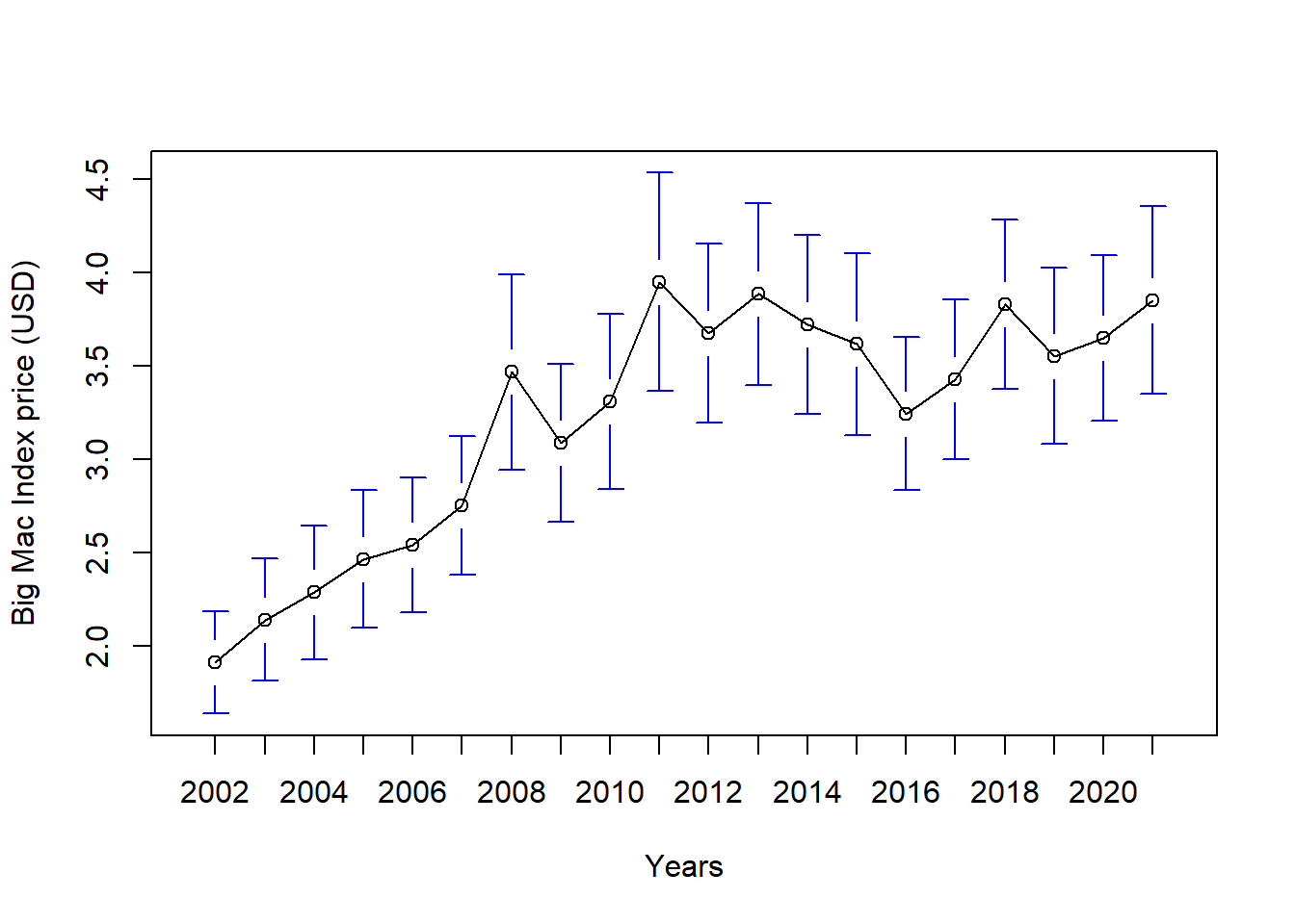
By Year
code block
plotmeans(bmi_usd_price~year, data = bmi_data, n.label=FALSE,xlab="Years",ylab="Big Mac Index price (USD)")
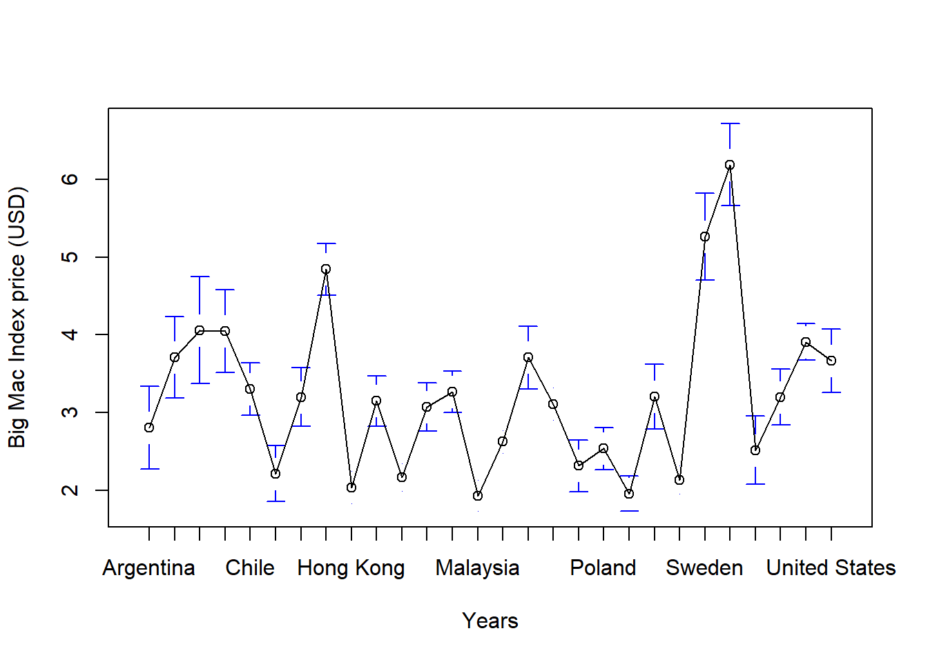
By Country
code block
plotmeans(bmi_usd_price~country, data = bmi_data, n.label=FALSE,xlab="Years",ylab="Big Mac Index price (USD)")
Note
Insights
We can see from the above plots that there is no homogeneity across years and countries. Hence, we should use heterogeneous panel data models.
The FE-model determines individual effects of unobserved, independent variables as constant (“fix“) over time. Within FE-models, the relationship between unobserved, independent variables and the IVs (i.e. endogeneity) can be existent.
Moreover,
FE remove the effect of those time-invariant characteristics so we can assess the net effect of the predictors on the outcome variable.
Another important assumption of the FE model is that those time-invariant characteristics are unique to the individual and should not be correlated with other individual characteristics. Each entity is different therefore the entity’s error term and the constant (which captures individual characteristics) should not be correlated with the others. If the error terms are correlated, then FE is no suitable since inferences may not be correct and you need to model that relationship (probably using random-effects).
Random Effects model
RE-models determine individual effects of unobserved, independent variables as random variables over time. They are able to “switch” between OLS and FE and hence, can focus on both dependencies between and withinindividuals.
Moreover,
An advantage of random effects is that you can include time invariant variables (i.e. gender). In the fixed effects model these variables are absorbed by the intercept. The cost is the possibility of inconsistent estimators, of the assumption is inappropriate.
Using the two statistically significant correlated variables of GDP per capita and HDI, we will create the panel regression to analyze the relationship with Big Mac Index prices.
Oneway (individual) effect Within Model

Call:
plm(formula = bmi_usd_price ~ gdp_per_capita + hdi, data = bmi_data,
    model = "within", index = c("country", "year"))

Balanced Panel: n = 28, T = 20, N = 560

Residuals:
      Min.    1st Qu.     Median    3rd Qu.       Max.
-1.9226068 -0.2728133  0.0086767  0.2729549  1.7410149

Coefficients:
                 Estimate Std. Error t-value  Pr(>|t|)
gdp_per_capita 7.6110e-05 3.7399e-06 20.3507 < 2.2e-16 ***
hdi            6.1167e+00 8.9549e-01  6.8305 2.328e-11 ***
---
Signif. codes:  0 '***' 0.001 '**' 0.01 '*' 0.05 '.' 0.1 ' ' 1

Total Sum of Squares:    346.67
Residual Sum of Squares: 131.29
R-Squared:      0.62129
Adj. R-Squared: 0.60057
F-statistic: 434.742 on 2 and 530 DF, p-value: < 2.22e-16
code block
random <-plm(bmi_usd_price ~ gdp_per_capita+hdi, data=bmi_data, index=c("country", "year"), model="random") #fixed modelsummary(random)
Oneway (individual) effect Random Effect Model
   (Swamy-Arora's transformation)

Call:
plm(formula = bmi_usd_price ~ gdp_per_capita + hdi, data = bmi_data,
    model = "random", index = c("country", "year"))

Balanced Panel: n = 28, T = 20, N = 560

Effects:
                 var std.dev share
idiosyncratic 0.2477  0.4977  0.36
individual    0.4405  0.6637  0.64
theta: 0.8346

Residuals:
     Min.   1st Qu.    Median   3rd Qu.      Max.
-1.651317 -0.330083 -0.001211  0.268572  2.165632

Coefficients:
                  Estimate  Std. Error z-value  Pr(>|z|)
(Intercept)    -1.8743e+00  7.0452e-01 -2.6604  0.007804 **
gdp_per_capita  6.9024e-05  3.7777e-06 18.2714 < 2.2e-16 ***
hdi             4.0807e+00  8.9766e-01  4.5459  5.47e-06 ***
---
Signif. codes:  0 '***' 0.001 '**' 0.01 '*' 0.05 '.' 0.1 ' ' 1

Total Sum of Squares:    362.26
Residual Sum of Squares: 157.1
R-Squared:      0.56634
Adj. R-Squared: 0.56478
Chisq: 727.402 on 2 DF, p-value: < 2.22e-16
As seen above, FE and RE models’ independent variables (GDP per capita and HDI) both have significant influence on BMI prices. Moreover, both models are good to use as their p-values are below alpha = 0.05. The Adjusted R-square variables are high with FE model having a higher value at 60% which means it represents the portion of the total variation in BMI prices that is explained by GDP per capita and HDI.
To determine between FE and RE models, we can use the Hausman-Test:
By running the Hausman-Test, the null hypothesis is that the covariance between IV(s) and alpha is zero. If this is the case, then RE is preferred over FE. If the null hypothesis is not true, we must go with the FE-model.
code block
phtest(fixed,random) #Hausman test
    Hausman Test

data:  bmi_usd_price ~ gdp_per_capita + hdi
chisq = 140.39, df = 2, p-value < 2.2e-16
alternative hypothesis: one model is inconsistent
Note
Insights
Given that the p-value is significant (<0.05), we reject the null hypothesis and can conclude that the fixed effects model is better.
6.2.3 Testing between FE and OLS models
To determine between FE and OLS (simple regression) models, we can use the pFtest to see which one is a better fitted model.
code block
pFtest(fixed, ols)
    F test for individual effects

data:  bmi_usd_price ~ gdp_per_capita + hdi
F = 45.056, df1 = 27, df2 = 530, p-value < 2.2e-16
alternative hypothesis: significant effects
Note
Given that the null hypothesis is that OLS is better fit model than Fixed Effect, the p-value is really small which means we reject the null hypothesis and can conclude that a FE model is a better fit.
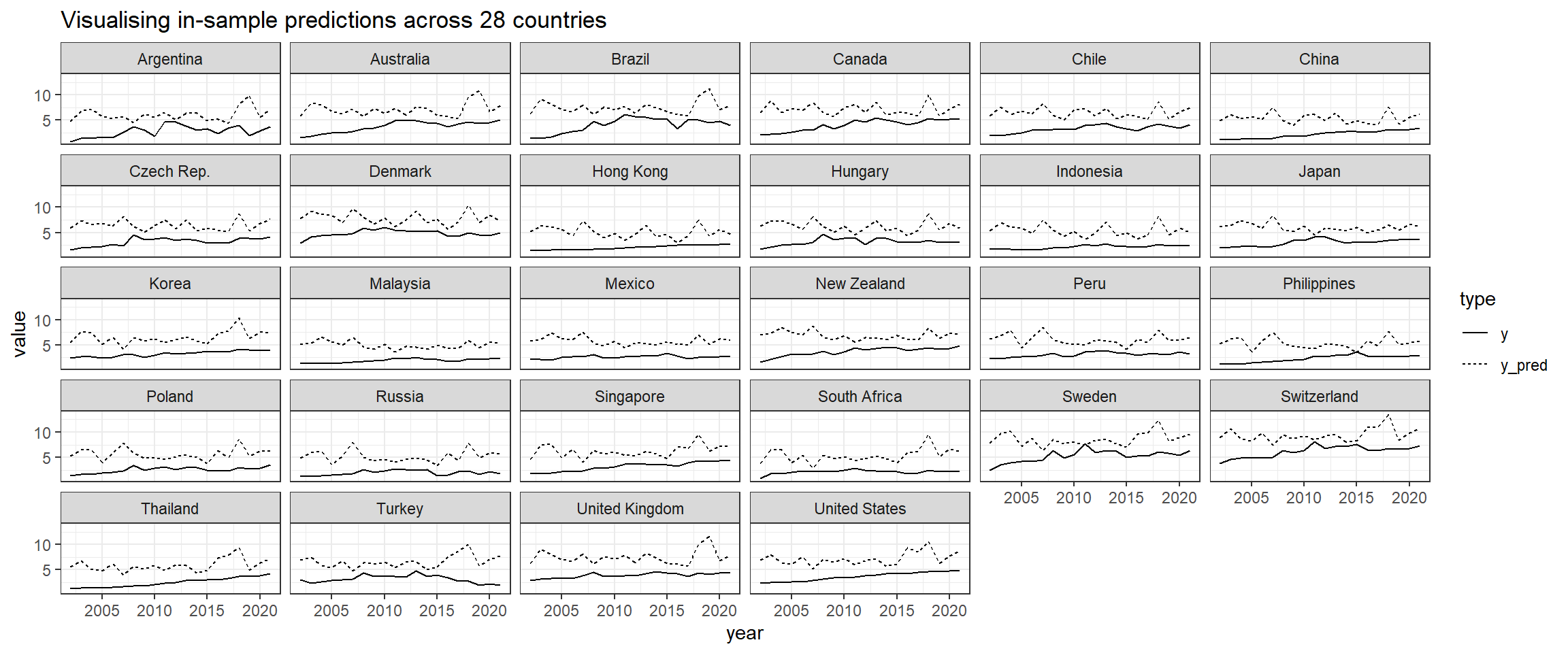
6.2.4 FE Model Diagnostics: Plotting predicted vs expected values
After conducting panel data regression, plotting predicted vs expected values allows us to visually assess the accuracy of your model’s predictions. The plot helps us identify any patterns or discrepancies between the predicted values from the Fixed Effects regression model and the actual observed values. It helps us validate the performance of the model and ensure it captures the underlying relationships effectively.
code block
## produce a dataset of prediction, added to the group meansbmi_means <- bmi_data %>%mutate(y = bmi_usd_price) %>%group_by(country) %>%transmute(y_mean =mean(y),y = y, year = year) %>%ungroup() %>%mutate(y_pred =predict(fixed) + y_mean) %>%select(-y_mean)## plot itbmi_means %>%gather(type, value, y, y_pred) %>%ggplot(aes(x = year, y = value, linetype = type))+geom_line() +facet_wrap(~country) +ggtitle("Visualising in-sample predictions across 28 countries")
Note
Insights
As we can see from the plots above, even though the Adjusted Rsquared for this model is 0.60, its predicted values are consistently higher than the observed y values. This means the model is not effectively capturing the relationships at each panel. Perhaps this poor model performance can be improved with clustering the countries - two different types of clusters (network clustering and time-series clustering) will be provided by my groupmates Firdaus and Jiayi respectively and added into the final Shiny app.
7 Conclusion
In conclusion, we used visualizations to explore the Big Mac Index prices for 28 countries across 20 years of 2002 to 2021. Visually, using univariate analysis, our plots depicted different trajectories in BMI prices across countries and a general upward trend across the years. When both dimensions were combined, we realised that there was an interaction effect between years and countries, and that there were 3 types of relationships ( positive, weak/zero, negative) between BMI prices and years when conditioned on countries.
This was further expanded in the visual time-series analysis that showed several outlier countries such as Hong Kong, Mexico, Russia, South Africa and Turkey. We could also see that when GDP per Capita was plotted against BMI prices, there seemed to be two groups of countries with different trajectories.
Thus, we conducted multivariate analysis to check which variables influenced Big Mac Index prices (putting aside year and country effects). There were interesting patterns e.g. those with large population sizes tended to have lower Big Mac Index prices. However, when statistically tested in a correlation plot, only GDP per capita and Human Development Index were statistically significantly correlated with BMI prices.
Despite our initial claim that the Big Mac Index is a proxy for inflation, our visual and statistical multivariate analyses did not support this claim.
With these variables, we conducted panel data regression analysis to confirm our analysis. Given the heterogeneity of data across years and countries, we cannot use homogeneous panel data models like OLS regression. Instead, through statistical analysis, Fixed Effect regression model is most suitable to explain the variation in BMI prices is explained by GDP per capita and HDI when we account for year and country effects.
8 Storyboard
For my part that comprised exploratory data analysis with univariate and time-series analysis, and confirmatory data analysis with panel data regression, my part in the Shiny web application is developed into the main dashboard, panel data analysis page under the Data Exploration analysis, and panel data regression under the Modelling page.
8.1 Dashboard (Summary)
The first section will consist of a homepage tab that allows users to select a country and year that the user is interested in. With a chloropleth map as the main focus (please refer to my groupmate Firdaus’s Take-home Exercise 4), a lollipop graph and violin+boxplot graph will be placed next to the chloropleth graph. Through this, the user is able to obtain a basic understanding on the individual country’s economic information, their BMI prices in relation to other countries and their BMI prices in relation to other years giving them the overall feel on how the BMI prices vary between countries and years and other information on their economic measures (that are later used for analysis).
Also, upload and export buttons are included for users to import data and export data of a fixed format. With the upload feature, any data uploaded by users will be automatically transformed and immediately analysed in the application. The export button allows the analysis and forecasted results to be exported in data or report format.
Proposed layout of Dashboard
The figure below shows some of the interactive features that will be incorporated into the dashboard. Users will have an overview of the BMI prices during their selected year with four key indicators.
Proposed interactive features of Dashboard
8.2 Panel Data Analysis (Data Exploration)
This section will be created using the ExPanD package that allows for interactive panel data exploration and analyses. Throughout the application, users will be able to select what variables they are interested in and tweak the plots to explore different parameters. After this section, the user will have a clearer understanding on the variables that influence BMI prices and the effects of time and countries on these relationships.
8.3 Panel Data Regression (Modelling)
This section will be also be created using the ExPanD package that allows for interactive panel data exploration and analyses. In this section, it showcases the statistical analysis on the variables that can explain the variation in BMI prices. Users will be able to vary the (multiple) variables in the panel regression analysis and see the results in the table. There will also be options to change the type of panel data regression and to select different clusters e.g. clusters from my groupmates Firdaus’ and Jiayi’s clustering analysis. At the bottom, ExPanD does not allow for custom addition of other plots so I will manually paste the predicted vs observed values plots according to no cluster, network cluster and time-series cluster.p;[
8.4 Conclusion
This section shows the initial prototype of the web application that we are planning to build to analyse and predict Big Mac Index prices.
Dashboard for Analysis and Prediction: The web application will serve as a dashboard where users can perform exploratory analysis, modelling and predicting of Big Mac Index prices.
Customizable Filters: The dashboard will include various filters such as selected periods and countries used for panel data analysis. These filters will allow users to customize their analysis based on their specific needs and preferences.
Personalized User Experience: The inclusion of customizable filters adds a personal touch to the user experience, allowing users to tailor their analysis to suit their individual requirements.
Overall, the web application aims to provide users with a powerful tool for analyzing and predicting Big Mac Index prices, leveraging customizable analysis features to enhance user experiences and provide valuable insights.
Source Code
---title: "Take-home Exercise 4"subtitle: "Take-home Exercise 4: [Prototyping Modules for Visual Analytics Shiny Application](https://isss608-ay2023-24jan.netlify.app/take-home_ex/th_ex04)" author: "Victoria Neo"date: 02/29/2024date-modified: last-modifiedformat: html: code-fold: true code-summary: "code block" code-tools: true code-copy: trueexecute: eval: true echo: true freeze: true warning: false message: false---{fig-align="left" width="630"}# 1 OverviewAs mentioned in my group's [proposal](https://isss608-24jan-group1.netlify.app/proposal/proposal),The [Big Mac Index](https://en.wikipedia.org/wiki/Big_Mac_Index) (BMI) was invented by [The Economist](https://www.economist.com/big-mac-index) in 1986 as a light-hearted guide to whether currencies are at their “correct” level. It is based on the theory of purchasing-power parity (PPP), with the notion that in the long run, exchange rates should move towards the rate that would equalise the prices of an identical basket of goods and services (in this case, a burger) in any two countries. The BMI has become a global standard, included in several economic textbooks and the subject of dozens of academic studies. Thus, we would like to visually examine the phenomenon of inflation co-movement by looking at the similarities in BMI prices between countries through time, isolate groups with similar characteristics, and determine if the BMI is a suitable proxy to inflation prices.There is a significant gap in making complex economic data accessible to the general public and providing advanced analysis tools for professionals. Existing visualization tools, including government dashboards, often fail to cater effectively to both audiences. To address this, we propose an R Shiny-based interactive tool that leverages publicly available data, the Big Mac Index to simplify the understanding of global financial trends for laypersons while offering in-depth data exploration and modelling capabilities for analysts.# 2 **Getting Started**## 2.1 Installing and loading the required libraries- [**AER**](https://cran.r-project.org/web/packages/AER/AER.pdf): for functions used in Applied Econometrics with R- **CGPfunctions**: for using `newggslopegraph()` for creating slopegraphs- [**corrplot**](https://cran.r-project.org/web/packages/corrplot/vignettes/corrplot-intro.html): provides a visual exploratory tool on correlation matrix that supports automatic variable reordering to help detect hidden patterns among variables.- [**dplyr**](https://dplyr.tidyverse.org/): for manipulating, concatenating dataframes- [**gplot**](https://cran.r-project.org/web/packages/gplots/gplots.pdf): for using `coplot()` for creating coplots- [**ggExtra**](https://cran.r-project.org/web/packages/ggExtra/vignettes/ggExtra.html): for adding marginal histograms to ggplot2- [**ggHoriPlot**](https://rivasiker.github.io/ggHoriPlot/): for plotting horizon plots- [**ggiraphExtra**](https://cran.r-project.org/web/packages/ggiraphExtra/index.html): for using ggPredict`()` for creating interactive multiple linear regression plots- [**ggpmisc**](https://cran.r-project.org/web/packages/ggpmisc/vignettes/model-based-annotations.html)**:** for using `stat_poly_eq()` for creating linear regression equations- [**ggstatsplot**](https://indrajeetpatil.github.io/ggstatsplot/): is an extension of [`{ggplot2}`](https://github.com/tidyverse/ggplot2) package for creating graphics with details from statistical tests- [**kableExtra**](https://cran.r-project.org/web/packages/kableExtra/vignettes/awesome_table_in_html.html)**,** for creating and manipulating complex tables- [**lubridate**](https://lubridate.tidyverse.org/): for using [`dmy()`](https://lubridate.tidyverse.org/reference/ymd.html) function to parse the Date field into appropriate Date data type in R- [**packHV**](https://cran.r-project.org/web/packages/packHV/packHV.pdf): for using `hist_boxplot()` for creating histograms with boxplots- [**patchwork**](https://cran.r-project.org/web/packages/patchwork/vignettes/patchwork.html)**:** for combining multiple ggplot2 graphs into one figure- [**parallelPlot**](https://cran.r-project.org/web/packages/parallelPlot/parallelPlot.pdf): for plotting Parallel Coordinates plots- [**plm**](https://cran.r-project.org/web/packages/plm/plm.pdf): for creating linear regression plots for panel data- [**purrr**](https://purrr.tidyverse.org/): for handling lists and functional programming- [**naniar**](https://cran.r-project.org/web/packages/naniar/vignettes/getting-started-w-naniar.html): for using `miss_vis()` function to check data for missing values- [**plotly**](https://plotly.com/r/): to make interactive graphs- [**tidyverse**](https://www.tidyverse.org/), a family of modern R packages specially designed to support data science, analysis and communication task including creating static statistical graphs```{r}pacman::p_load(AER, CGPfunctions, corrplot, dplyr, DT, gplots, ggExtra, ggHoriPlot, ggiraphExtra, ggpmisc, ggthemes, ggplot2, ggstatsplot, kableExtra, lubridate, packHV, patchwork, parallelPlot, plm, purrr, naniar, plotly, tidyverse ) ```## 2.2 **Data Set**### 2.2.1 Loading the Data SetWe load the dataset for Big Mac Index that has been combined with other data (e.g. GDP, Employment rates etc.) and the country dataset as seen here in our [data preparation](https://isss608-24jan-group1.netlify.app/prototype/data_preparation/data_preparation). We left join the country dataset to the Big Mac Index dataset.```{r}indicator_data <-read_csv("data/countries_with_complete_data.csv")``````{r}country_data <-read_csv("data/country_all.csv")``````{r}bmi_data <-left_join(indicator_data, country_data, by =c("country"))```### 2.2.2 Checking Data HealthWe now check the health of our dataset by using:- `datatable()` from the DT package to view the dataframe more interactively,- `glimpse()` to look at the structure of the dataframe, data types of the columns, and some values of the dataframe,- `duplicate()` to check the dataframe for any duplicated entries using *duplicate()*, and- `vis_miss()` to check the state of missing values in the dataset.- `describe()` to produce a summary of all the variables.::: panel-tabset## **datatable()**```{r}datatable(bmi_data, class="compact",rownames =FALSE,width="100%", options =list(pageLength =10,scrollX=T))```## **glimpse()**```{r}glimpse(bmi_data)```## **duplicate()**```{r}bmi_data[duplicated(bmi_data),]```## **vis_miss()**```{r}vis_miss(bmi_data)```## **describe()**```{r}Hmisc::describe(bmi_data)```:::### 2.2.3 Descriptive StatisticsWe now summarize our dataset by using:- a function for categorical variables- `summary()` for continuous variables::: panel-tabset## **fun_cat for categorical variables**```{r}fun_cat <-function(x) {# Count the number of missing values nmiss <-sum(is.na(x))# Frequency n <-table(x)# Proportion p <-prop.table(n)# Putting it together OUT <-cbind(n, p)# Add nmiss, but first pad to have the right number of rows nmiss <-c(nmiss, rep(NA, nrow(OUT)-1)) OUT <-cbind(OUT, nmiss)return(OUT)}```## **Categorical variables**```{r}fun_cat(bmi_data$country)fun_cat(bmi_data$currency_code)fun_cat(bmi_data$year)fun_cat(bmi_data$continent)fun_cat(bmi_data$g20)fun_cat(bmi_data$brics)fun_cat(bmi_data$eu)```## **Continuous variables**```{r}cont_data <-data.frame(bmi_data$bmi_localprice, bmi_data$bmi_usd_price, bmi_data$bot, bmi_data$gdp, bmi_data$gdp_per_capita, bmi_data$inflation, bmi_data$hdi, bmi_data$population)lapply(cont_data, summary)```## **bmi_usdprice by year**```{r}# Assuming 'bmi_data' is your data frameresult_list <-lapply(split(bmi_data, bmi_data$year),function(sub_data) summary(sub_data$bmi_usd_price))result_list```## **bmi_usdprice by country**```{r}# Assuming 'bmi_data' is your data frameresult_list <-lapply(split(bmi_data, bmi_data$country),function(sub_data) summary(sub_data$bmi_usd_price))result_list```:::# 3 **Exploratory Data Analysis**```{mermaid}flowchart TB A[Year] B[Country] C[Big Mac Index price] D[Inflation rate] E[GDP per capita] F[Balance of Trade] G[Unemployment rate] H[Human Development Index] I[Population size] A --> C B --> C C --> D C --> E C --> F C --> G C --> H C --> I```Some questions of interest regarding the problem statement of inflation co-movement by BMI are:- what type of variation occurs within BMI prices,- what type of covariation occurs between BMI prices by dimensions.To do this, we will look at the following variables:1. bmi_usd_price (in order to compare across currencies, we use the BMI prices converted to USD)by dimensions1. country2. year## 3.1 Univariate Analysis: Looking at BMI```{r}par(mfrow =c(1, 2))hist_boxplot(bmi_data$bmi_usd_price,col="#69b3a2",freq=TRUE, xlab ="Prices in USD", main ="Histogram of Big Mac Index prices in USD")hist_boxplot(bmi_data$bmi_usd_price,col="#69b3a2",freq=FALSE,density=TRUE, xlab ="Prices in USD", main ="")```::: callout-note### **Insights**BMI is asymmetrically distributed and skewed to the right. Most of the Big Mac prices (adjusted to USD) are close to 3USD - this makes sense as McDonald's positions itself as an ultra-affordable fast food chain. Its mean (3.2198) is higher than its median (2.9915). But this also means that it has outliers with very expensive Big Mac prices.Questions:- Why are the Big Mac prices close to 3USD?- Given McDonald's strategy to be ultra-affordable, why is there a large spread in Big Mac prices and outliers on the right?:::## 3.2 Looking at BMI through individual dimensions### 3.2.1 Country dimension **with Violin+Boxplot**```{r, fig.height = 8}bmi_data %>% # Calculate mean of bmi_usd_price for each country group_by(country) %>% mutate(median_bmi = median(bmi_usd_price)) %>% ungroup() %>% # Reorder the countries based on the mean of bmi_usd_price mutate(country = reorder(country, median_bmi)) %>% # Add a column called 'type': do we want to highlight the group or not? mutate(type = ifelse(country=="United States", "Highlighted", "Normal")) %>% # Build the boxplot. ggplot(aes(x = country, y = bmi_usd_price, fill = type, alpha = type)) + geom_violin(width=1.0) + geom_boxplot(width=0.3, color="black", alpha=0.8) + geom_jitter(color = "black", size = 0.4, alpha = 0.9) + scale_fill_manual(values = c("#69b3a2", "grey")) + scale_alpha_manual(values = c(1, 0.1)) + theme(legend.position = "none") + labs(y = "Prices in USD", x = "", title = "Boxplot of Big Mac Index Prices in USD across countries") + coord_flip() + # Add mean and median lines geom_hline(aes(yintercept = mean(bmi_usd_price), linetype = "Mean"), color = "darkblue", linetype = "dashed", size = 0.5) + geom_hline(aes(yintercept = median(bmi_usd_price), linetype = "Median"), color = "darkred", linetype = "dashed", size = 0.5) + # Add text labels for mean and median geom_text(aes(x = mean(bmi_usd_price), label = paste("Mean: ", round(mean(bmi_usd_price), 2))), y = max(bmi_data$bmi_usd_price, na.rm = TRUE), size = 3, vjust =3.5, hjust = 1, color = "darkblue") + geom_text(aes(x = median(bmi_usd_price), label = paste("Median: ", round(median(bmi_usd_price), 2))), y = max(bmi_data$bmi_usd_price, na.rm = TRUE), size = 3, vjust = 4, hjust = 1, color = "darkred") + # Customize legend scale_linetype_manual(name = "Lines", values = c("Mean" = "dashed", "Median" = "dashed"), labels = c("Mean", "Median")) + guides(fill = guide_legend(override.aes = list(alpha = c(1, 0.1)))) ```::: callout-note### **Insights**Some of the outliers pointed out in the previous data visualisations can be explained by the country dimension. Highly developed countries such as Switzerland, Sweden and Denmark have the top 3 most expensive Big Mac prices. However, Hong Kong, with also a highly developed economy, has the third lowest Big Mac price. In the boxplot above, there is no clear difference between developed and developing countries (even Philippines is more expensive than Hong Kong).The above boxplot also shows that there is variation within and between countries - there are some countries with greater variability e.g. Argentina and a number of countries with median BMI prices higher than the overall median BMI price such as Switzerland, Brazil and Canada while countries like Mexico and South Africa (somewhat bimodal) did not see much fluctuations in their BMI prices.Questions:- Why do some countries have greater variability in their BMI prices?- Why is there a difference in BMI prices between developed and developing countries? - especially for Hong Kong:::### 3.2.2 Year dimension with Violin+Boxplot```{r, fig.height = 8}bmi_data %>% mutate(year = factor(year)) %>% # Add a column called 'type': do we want to highlight the group or not? mutate( type=ifelse(year %in% c("2002", "2021"),"Highlighted","Normal")) %>% # Build the boxplot. In the 'fill' argument, give this column ggplot( aes(x=year, y=bmi_usd_price, fill=type, alpha=type)) + geom_violin(width=1.0) + geom_boxplot(width=0.3, color="black", alpha=0.8) + geom_jitter(color = "black", size = 0.4, alpha = 0.9) + scale_fill_manual(values=c("#69b3a2", "grey")) + scale_alpha_manual(values=c(1,0.1)) + theme(legend.position = "none") + labs(y = "Prices in USD", x = "", title = "Boxplot of Big Mac Index Prices in USD across years") + coord_flip() + # Add mean and median lines geom_hline(aes(yintercept = mean(bmi_usd_price), linetype = "Mean"), color = "darkblue", linetype = "dashed", size = 0.5) + geom_hline(aes(yintercept = median(bmi_usd_price), linetype = "Median"), color = "darkred", linetype = "dashed", size = 0.5) + # Add text labels for mean and median geom_text(aes(x = mean(bmi_usd_price), label = paste("Mean: ", round(mean(bmi_usd_price), 2))), y = max(bmi_data$bmi_usd_price, na.rm = TRUE), size = 3, vjust =3.5, hjust = 1, color = "darkblue") + geom_text(aes(x = median(bmi_usd_price), label = paste("Median: ", round(median(bmi_usd_price), 2))), y = max(bmi_data$bmi_usd_price, na.rm = TRUE), size = 3, vjust = 4, hjust = 1, color = "darkred") + # Customize legend scale_linetype_manual(name = "Lines", values = c("Mean" = "dashed", "Median" = "dashed"), labels = c("Mean", "Median")) + guides(fill = guide_legend(override.aes = list(alpha = c(1, 0.1)))) ```::: callout-note### **Insights**From the boxplot above, we can see that Big Mac prices have risen through the years - 2021 is the most expensive year for Big Mac prices. Moreover from 2002 - 2007, according to the violin plot, it seemed that the prices were mostly concentrated but there is more spread since 2008. Despite the blip from 2013 - 2016 and 2018 - 2020, which saw falling Big Mac prices, as a whole, they have increased since 2002 which saw the lowest prices for Big Mac.Questions:- Why was there a dip in Big Mac prices from 2013 to 2016 and 2018 to 2020?- Why are Big Mac prices rising as a whole?:::## 3.3 Looking at BMI through both dimensions### 3.3.1 Plotting a Coplot plot to determine if there is a third variable influenceThe BMI price in USD is plotted on the y axis and the years are on the x axis. The 28 plots show the relationship between these two variables by each country. The bars at the top indicate the countries position from left to right, starting from the bottom row.```{r, fig.width = 12}coplot(bmi_usd_price ~ year|country, data = bmi_data, panel = function(x, y, ...) { points(x, y, ...) abline(lm(y ~ x), col = "blue")})```::: callout-note**Insights**From the coplots above, there is an interaction between years and countries. Conditionally on country, the relationship between BMI price in USD and year looks roughly linear - the regression results for most countries indicate a positive relationship throughout the years. However, countries like Hong Kong(11), Mexico(15), Russia(20) and South Africa(22) have almost flat regression lines that suggest a weak or almost no relationship between the variables. Moreover, Turkey(26) is the only country with a negative relationship.:::# 4 **Time-series Analysis of Big Mac Index through time and countries**## 4.1 Looking at overall trends with `newsslopegraph()````{r, fig.width= 10, fig.height = 15}bmi_data %>% mutate(year = factor(year)) %>% filter(year %in% c(2002, 2011, 2021 )) %>% newggslopegraph(year, bmi_usd_price, country, Title = "Big Mac Index (USD) across 28 countries", SubTitle = "At 10 Years Intervals from 2002-2021", Caption = "Source: The Economist", YTextSize = 2.5, LineThickness = .6, LineColor = c(rep("gray",8), "red", rep("gray",18), "#69b3a2"), WiderLabels = TRUE)```::: callout-note### **Insights**From the slopegraph above, we can see that Big Mac prices increased for all countries in 2011 but later increased for some and decreased for others. Switzerland consistently had the most expensive Big Mac prices through the years while Argentina had the cheapest Big Mac in 2002 but is in 15th position (out of 28) in 2021. Most interesting is Hong Kong, that saw a consistent rise in Big Mac process, did not experience sharp changes, and had actually the cheapest Big Mac in 2011.Moreover, in 2002, the prices between countries were much closer in spread but this spread increased through the years.Questions:- Why did the spread in Big Mac prices between countries increase through the years?- Why did Big Mac prices increase in 2011 for all countries?- Why did some countries experience a consistent increase in Big Mac prices while others experienced fluctuations?:::## 4.2 Looking at variations in patterns with `ggHoriPlot()`Toggle the different tabsets to see the different horizon plots.::: panel-tabset## **using United States mean bmi_usd_price as the baseline**```{r}mean_us_bmi_price <- bmi_data %>%filter(country =="United States") %>%summarise(mean_bmi_usd_price =mean(bmi_usd_price, na.rm =TRUE))mean_us_bmi_pricebmi_data %>%filter(year >="2002") %>%ggplot() +geom_horizon(aes(x = year, y=bmi_usd_price), origin =3.666, horizonscale =6)+facet_grid(`country`~.) +theme_few() +scale_fill_hcl(palette ='RdBu') +theme(panel.spacing.y=unit(0, "lines"), strip.text.y =element_text(size =5, angle =0, hjust =0),legend.position ='none',axis.text.y =element_blank(),axis.text.x =element_text(size=7),axis.title.y =element_blank(),axis.title.x =element_blank(),axis.ticks.y =element_blank(),panel.border =element_blank() ) ```If US mean bmi_usd_price is used as the origin, Switzerland (and shortly after) Denmark have always had stronger prices than the overall mean Big Mac Index price for USA. China, Hong Kong, Indonesian, Malaysia, Mexico, Philippines, Poland, Russia, South Africa and Turkey have always been weaker in Big Mac prices than the USA.## **using mean bmi_usd_price as the baseline**```{r}bmi_data %>%filter(year >="2002") %>%ggplot() +geom_horizon(aes(x = year, y=bmi_usd_price), origin ="mean", horizonscale =6)+facet_grid(`country`~.) +theme_few() +scale_fill_hcl(palette ='RdBu') +theme(panel.spacing.y=unit(0, "lines"), strip.text.y =element_text(size =5, angle =0, hjust =0),legend.position ='none',axis.text.y =element_blank(),axis.text.x =element_text(size=7),axis.title.y =element_blank(),axis.title.x =element_blank(),axis.ticks.y =element_blank(),panel.border =element_blank() ) ```## **using median bmi_usd_price as the baseline**```{r}bmi_data %>%filter(year >="2002") %>%ggplot() +geom_horizon(aes(x = year, y=bmi_usd_price), origin ="median", horizonscale =6)+facet_grid(`country`~.) +theme_few() +scale_fill_hcl(palette ='RdBu') +theme(panel.spacing.y=unit(0, "lines"), strip.text.y =element_text(size =5, angle =0, hjust =0),legend.position ='none',axis.text.y =element_blank(),axis.text.x =element_text(size=7),axis.title.y =element_blank(),axis.title.x =element_blank(),axis.ticks.y =element_blank(),panel.border =element_blank() ) ```:::::: callout-note### **Insights**The horizon plot (**using median bmi_usd_price as the baseline)** showed that all countries were initially below the median Big Mac price and all experienced some increase in price. China, Hong Kong, Korea, Singapore, Thailand and United States had a huge increase in Big Mac prices around 2018 to 2022. However, Turkey experienced a large drop in recent years while Russia experienced huge increase and than a large drop around 2015 and only had a smaller increase later on.Questions:- Why do some countries experience a significant increase in Big Mac prices together over the same period?- Why are there small sharp peaks for some years and long peaks for others?- What other factors account for this co-movement in Big Mac prices? GDP per capita?:::## 4.3 Adding GDP per capita to track the movement of BMI through the years, countries (colour) and population (size) with a Bubble Plot```{r}bmi_data %>%plot_ly(x =~gdp_per_capita, y =~bmi_usd_price, size =~population, color =~country,sizes =c(20, 150),frame =~year, text =~paste(country, "<br>Population: ", gdp_per_capita, "<br>Big Mac Price: USD$", bmi_usd_price,"<br>GDP per Capita: $", gdp_per_capita, "<br>Inflation: ", inflation, "%"), hoverinfo ="text",type ='scatter',mode ='markers' ) %>%layout(showlegend =FALSE,xaxis =list(title ="GDP per Capita"),yaxis =list(title ="Price in USD"),title ="A Bubbleplot of Big Mac Index (USD) across 28 countries (colour) with population (size) through the years")```::: callout-note### **Insights**At the start, it seemed like there was a relationship between GDP per capita and BMI prices - the higher one's GDP per capita was, the higher the Big Mac price in USD. Switzerland with the highest GDP per capita also saw the most expensive Big Mac prices. The only exception is Hong Kong that had a small inflation rate throughout. For those with higher GDP per capita, their inflation rates were almost the same. While countries with higher GDP per capita above 40k saw their GDP per capita increasing with Big Mac prices consistently above USD\$3 since 2010, countries with GDP per capita below 20k saw small increases in their GDP per capita, still remained below 20k while Big Mac prices had a wider variability. Also, most of the countries in our study are of the similar population size.Questions:- There seems to be two different trajectory of BMI prices for countries with different GDP per capita. Are there other factors influencing this? Are there other trajectories that can be seen?- We have been mostly looking at country and year effects. Are there other variables that affect BMI as a whole?:::# 5 **Multivariate Analysis of Big Mac Index through time and countries**## 5.1 Plotting a Parallel Coordinates plot to see relationships between variables```{r, fig.width=12, fig.height=10}pc <- bmi_data %>% select( gdp_per_capita, bot, inflation, unemployment, hdi, population, bmi_usd_price)histoVisibility <- rep(TRUE, ncol(pc))parallelPlot(pc, histoVisibility = histoVisibility)```::: callout-note**Insights**Based on the parallel coordinates plot, there appears to be interesting patterns. For example, countries lower gdp_per-capita, higher balance of trade (net export - net import) with low inflation and unemployment, and big population sizes had low Big Mac Index prices. Countries with high gdp_per_capita with high human development index (HDI) and small population sizes had very high Big Mac Index prices.Questions:- What are the correlations between variables with BMI in USD prices?:::## 5.2 Plotting a Correlation plot to see correlations between variables```{r, fig.width = 12}columns_of_interest <- c("gdp_per_capita", "bot", "inflation", "unemployment", "hdi", "population", "bmi_usd_price")bmi.cor <- cor(bmi_data[, columns_of_interest])bmi.sig = cor.mtest(bmi.cor, conf.level= .95)corrplot(bmi.cor, method = "number", type = "lower", diag = FALSE, tl.col = "black", tl.srt = 45, p.mat = bmi.sig$p, sig.level = .05)```::: callout-note**Insights**GDP per capita, inflation and Human Development Index are significantly correlated to Big Mac Index prices. Interestingly, even though we had initially posited that inflation and Big Mac prices are correlated, it appears that they are not - inflation is not correlated to Big Mac Index prices. However, we cannot tell if there is a year/country effect - there is no information on the correlation even though though these variables are constant in the time dimension and across countries.:::# 6 Panel Data RegressionGiven the time-series (by 20 years) and cross sectionality (by 28 countries) of our data, panel data regression is a good technique to analyze the relationship between our independent variables and Big Mac Index price.## 6.1 Homogenous Panel Data modelFrom the article [**Introduction to the Fundamentals of Panel Data**](https://www.aptech.com/blog/introduction-to-the-fundamentals-of-panel-data/),> Homogeneous (or pooled) panel data models assume that the model parameters are common across individuals.Thus, the basic OLS regression model does not consider heterogeneity across countries or years.```{r}ols <-lm(bmi_usd_price ~ gdp_per_capita + hdi, data = bmi_data)summary(ols)``````{r, fig.width = 12, fig.height = 10}ggPredict(ols,interactive=TRUE)```::: callout-note**Insights**Each point represents observations of GDP per capita, HDI and BMI price in USD - the multiple regression results indicate a positive relationship throughout the years.. However, this cannot account for omitted unobservable factors that exist from country to country and year to year.:::## 6.2 Heterogeneous Panel Data modelsFrom the article [**Introduction to the Fundamentals of Panel Data**](https://www.aptech.com/blog/introduction-to-the-fundamentals-of-panel-data/),> Heterogeneous models allow for any or all of the model parameters to vary across individuals. Fixed effects and random effects models are both examples of heterogeneous panel data models.### 6.2.1 Testing for Heterogeneity across Year and Country**By Year**```{r}plotmeans(bmi_usd_price~year, data = bmi_data, n.label=FALSE,xlab="Years",ylab="Big Mac Index price (USD)")```**By Country**```{r}plotmeans(bmi_usd_price~country, data = bmi_data, n.label=FALSE,xlab="Years",ylab="Big Mac Index price (USD)")```::: callout-note**Insights**We can see from the above plots that there is no homogeneity across years and countries. Hence, we should use heterogeneous panel data models.:::### 6.2.2 Choosing which model is appropriateDefinitions of different models taken from the articles [**A Guide to Panel Data Regression: Theoretics and Implementation with Python**](https://towardsdatascience.com/a-guide-to-panel-data-regression-theoretics-and-implementation-with-python-4c84c5055cf8)and [**Panel Data Using R: Fixed-effects and Random-effects**](https://libguides.princeton.edu/R-Panel):1. Fixed Effects model > The FE-model determines individual effects of unobserved, independent variables as constant (“fix“) over time. Within FE-models, the relationship between unobserved, independent variables and the IVs (i.e. endogeneity) can be existent. > >  > > Moreover, > > **FE remove the effect of those time-invariant characteristics so we can assess the net effect of the predictors on the outcome variable.** > > Another important assumption of the FE model is that those time-invariant characteristics are unique to the individual and should not be correlated with other individual characteristics. Each entity is different therefore the entity’s error term and the constant (which captures individual characteristics) should not be correlated with the others. If the error terms are correlated, then FE is no suitable since inferences may not be correct and you need to model that relationship (probably using random-effects).2. Random Effects model > RE-models determine individual effects of unobserved, independent variables as random variables over time. They are able to “switch” between OLS and FE and hence, can focus on both dependencies **between** and **within** **individuals**. > >  > > Moreover, > > An advantage of random effects is that you can include time invariant variables (i.e. gender). In the fixed effects model these variables are absorbed by the intercept. The cost is the possibility of inconsistent estimators, of the assumption is inappropriate.Using the two statistically significant correlated variables of GDP per capita and HDI, we will create the panel regression to analyze the relationship with Big Mac Index prices.::: panel-tabset## **Fixed effects model**```{r}fixed <-plm(bmi_usd_price ~ gdp_per_capita+hdi, data=bmi_data, index=c("country", "year"), model="within") #fixed modelsummary(fixed)```## **Random effects model**```{r}random <-plm(bmi_usd_price ~ gdp_per_capita+hdi, data=bmi_data, index=c("country", "year"), model="random") #fixed modelsummary(random)```:::As seen above, FE and RE models' independent variables (GDP per capita and HDI) both have significant influence on BMI prices. Moreover, both models are good to use as their p-values are below alpha = 0.05. The Adjusted R-square variables are high with FE model having a higher value at 60% which means it represents the portion of the total variation in BMI prices that is explained by GDP per capita and HDI.To determine between FE and RE models, we can use the Hausman-Test:> By running the Hausman-Test, the null hypothesis is that the covariance between IV(s) and *alpha* is zero. If this is the case, then RE is preferred over FE. If the null hypothesis is not true, we must go with the FE-model.```{r}phtest(fixed,random) #Hausman test```::: callout-note**Insights**Given that the p-value is significant (\<0.05), we reject the null hypothesis and can conclude that the fixed effects model is better.:::### 6.2.3 Testing between FE and OLS modelsTo determine between FE and OLS (simple regression) models, we can use the pFtest to see which one is a better fitted model.```{r}pFtest(fixed, ols)```::: callout-noteGiven that the null hypothesis is that OLS is better fit model than Fixed Effect, the p-value is really small which means we reject the null hypothesis and can conclude that a FE model is a better fit.:::### 6.2.4 FE Model Diagnostics: Plotting predicted vs expected valuesAfter conducting panel data regression, plotting predicted vs expected values allows us to visually assess the accuracy of your model's predictions. The plot helps us identify any patterns or discrepancies between the predicted values from the Fixed Effects regression model and the actual observed values. It helps us validate the performance of the model and ensure it captures the underlying relationships effectively.```{r, fig.width=12}## produce a dataset of prediction, added to the group meansbmi_means <- bmi_data %>% mutate(y = bmi_usd_price) %>% group_by(country) %>% transmute(y_mean = mean(y), y = y, year = year) %>% ungroup() %>% mutate(y_pred = predict(fixed) + y_mean) %>% select(-y_mean)## plot itbmi_means %>% gather(type, value, y, y_pred) %>% ggplot(aes(x = year, y = value, linetype = type))+ geom_line() + facet_wrap(~country) + ggtitle("Visualising in-sample predictions across 28 countries")```::: callout-note**Insights**As we can see from the plots above, even though the Adjusted Rsquared for this model is 0.60, its predicted values are consistently higher than the observed y values. This means the model is not effectively capturing the relationships at each panel. Perhaps this poor model performance can be improved with clustering the countries - two different types of clusters (network clustering and time-series clustering) will be provided by my groupmates Firdaus and Jiayi respectively and added into the final Shiny app.:::# 7 ConclusionIn conclusion, we used visualizations to explore the Big Mac Index prices for 28 countries across 20 years of 2002 to 2021. Visually, using univariate analysis, our plots depicted different trajectories in BMI prices across countries and a general upward trend across the years. When both dimensions were combined, we realised that there was an interaction effect between years and countries, and that there were 3 types of relationships ( positive, weak/zero, negative) between BMI prices and years when conditioned on countries.This was further expanded in the visual time-series analysis that showed several outlier countries such as Hong Kong, Mexico, Russia, South Africa and Turkey. We could also see that when GDP per Capita was plotted against BMI prices, there seemed to be two groups of countries with different trajectories.Thus, we conducted multivariate analysis to check which variables influenced Big Mac Index prices (putting aside year and country effects). There were interesting patterns e.g. those with large population sizes tended to have lower Big Mac Index prices. However, when statistically tested in a correlation plot, only GDP per capita and Human Development Index were statistically significantly correlated with BMI prices.Despite our initial claim that the Big Mac Index is a proxy for inflation, our visual and statistical multivariate analyses did not support this claim.With these variables, we conducted panel data regression analysis to confirm our analysis. Given the heterogeneity of data across years and countries, we cannot use homogeneous panel data models like OLS regression. Instead, through statistical analysis, Fixed Effect regression model is most suitable to explain the variation in BMI prices is explained by GDP per capita and HDI when we account for year and country effects.# 8 StoryboardFor my part that comprised exploratory data analysis with univariate and time-series analysis, and confirmatory data analysis with panel data regression, my part in the Shiny web application is developed into the main dashboard, panel data analysis page under the Data Exploration analysis, and panel data regression under the Modelling page.## 8.1 Dashboard (Summary)The first section will consist of a homepage tab that allows users to select a country and year that the user is interested in. With a chloropleth map as the main focus (please refer to my groupmate Firdaus's Take-home Exercise 4), a lollipop graph and violin+boxplot graph will be placed next to the chloropleth graph. Through this, the user is able to obtain a basic understanding on the individual country's economic information, their BMI prices in relation to other countries and their BMI prices in relation to other years giving them the overall feel on how the BMI prices vary between countries and years and other information on their economic measures (that are later used for analysis).Also, upload and export buttons are included for users to import data and export data of a fixed format. With the upload feature, any data uploaded by users will be automatically transformed and immediately analysed in the application. The export button allows the analysis and forecasted results to be exported in data or report format.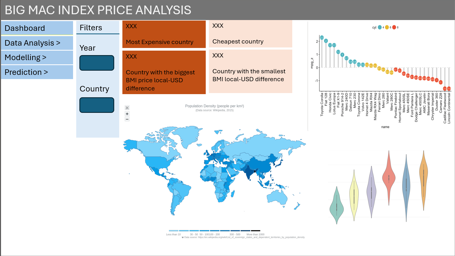{fig-align="left"}The figure below shows some of the interactive features that will be incorporated into the dashboard. Users will have an overview of the BMI prices during their selected year with four key indicators.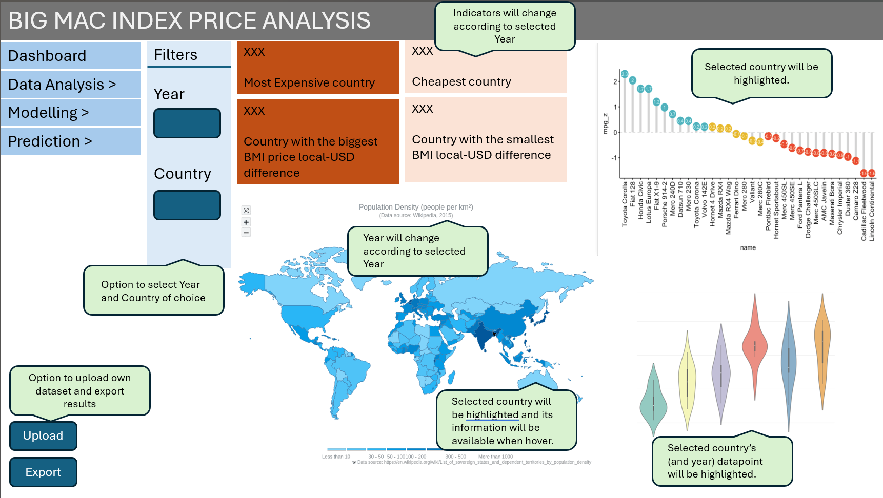## 8.2 Panel Data Analysis (Data Exploration)This section will be created using the ExPanD package that allows for interactive panel data exploration and analyses. Throughout the application, users will be able to select what variables they are interested in and tweak the plots to explore different parameters. After this section, the user will have a clearer understanding on the variables that influence BMI prices and the effects of time and countries on these relationships.## 8.3 Panel Data Regression (Modelling)This section will be also be created using the ExPanD package that allows for interactive panel data exploration and analyses. In this section, it showcases the statistical analysis on the variables that can explain the variation in BMI prices. Users will be able to vary the (multiple) variables in the panel regression analysis and see the results in the table. There will also be options to change the type of panel data regression and to select different clusters e.g. clusters from my groupmates Firdaus' and Jiayi's clustering analysis. At the bottom, ExPanD does not allow for custom addition of other plots so I will manually paste the predicted vs observed values plots according to no cluster, network cluster and time-series cluster.p;\[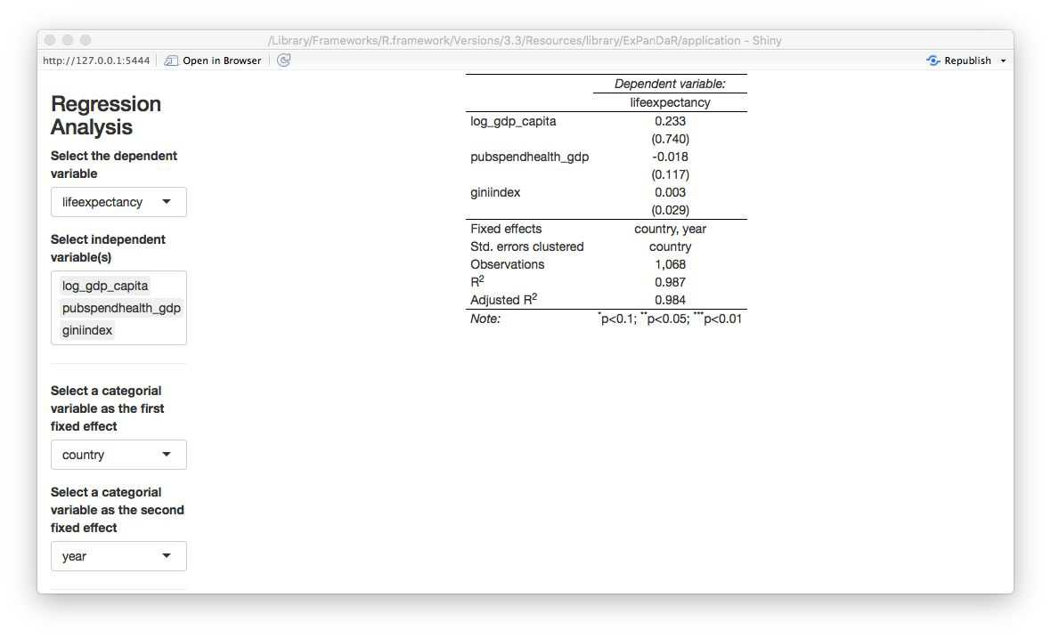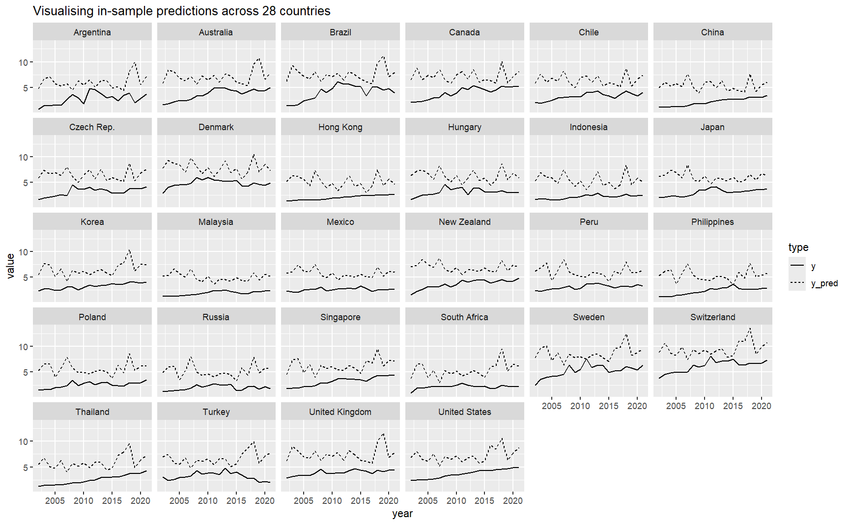## 8.4 ConclusionThis section shows the initial prototype of the web application that we are planning to build to analyse and predict Big Mac Index prices.1. **Dashboard for Analysis and Prediction**: The web application will serve as a dashboard where users can perform exploratory analysis, modelling and predicting of Big Mac Index prices.2. **Customizable Filters**: The dashboard will include various filters such as selected periods and countries used for panel data analysis. These filters will allow users to customize their analysis based on their specific needs and preferences.3. **Personalized User Experience**: The inclusion of customizable filters adds a personal touch to the user experience, allowing users to tailor their analysis to suit their individual requirements.Overall, the web application aims to provide users with a powerful tool for analyzing and predicting Big Mac Index prices, leveraging customizable analysis features to enhance user experiences and provide valuable insights.##